Markov Models

Markov assumption states that the probability of the current state depends only on a finite series of previous states. As a special case, this assumption gives rise to the Markov chain representation, asserting that future state predictions are conditionally independent of the past given the present state-$P(Xt | X{t-1})$

Hidden Markov Models

In hidden markov models, our agent usually don’t have a information about the state, , instead, our agents gather observations over time.

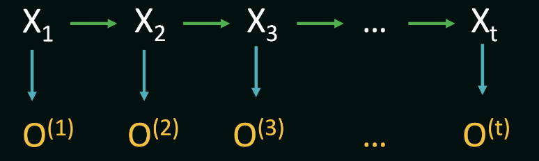
A Hidden Markov Model consists of three fundamental components: the initial distribution $P(X1)$, transition probabilities denoted by $P(Xt | X{t-1})$, and observation probabilities $P(O_t | X_t)$. Additionally, HMMs operate under two critical Markov assumptions:

The future states of the system depend solely on the present state, encapsulated by the transition probabilities $P(Xt | X{t-1})$.
The observation at a particular time step depend solely on the current state, encapsulated by the transition probabilities $P(O_t | X_t)$.

Compute the probability of an observation sequence

If we know the hidden state sequence, then the computation of the probability is straightforward.

$P(O | S) = P((o_1, o_2, \dots, o_T) | S) = \prod_{t=1}^{T}P(s_t|s_{t-1}) \cdot P(o_t | s_t)$

To compute $P(s_1 | s_0)$ in the above equation (the probability of being in a specific hidden state at the first time step), we often simply resort to using the stationary distribution of the Markov chain defined over the hidden states.

If we do not know the hidden state sequence, only know the observation sequence, then, in this scenario, we need to account for all possible hidden-state sequences, and sum over their joint probabilities with the observation sequence.

$P(O) = \sum_{S} P(O | S) P(S)$

However, if we do bruteforcely, for an HMM with $N$ hidden states and an observation sequence of $T$ observations, there are $N^T$ possible hidden sequences, which is unacceptable. To solve this problem, we can exploit the fact that the probability of the observation sequence up to time $t$ can be computed using the probability of the observation sequence up to time $t-1$. This is done by summing over the probabilities of all possible hidden-state sequences at time:

$P(O_{0 \to t} | (s_t= s_i)) = \sum_{j=1}^{N} P(O_{0 \to t-1} | (s_{t-1}=s_j))P(s_i|s_j)P(o_t|s_i)$

Then, we have

$P(O_{o \to t}) = \sum_{i=1}^{N} P(O_{0 \to t} | (s_t= s_i))$

Having the recurrance, we can use dynamic programming to solve this problem with a $O(N^2 T)$ time complexity. Still, at $t=1$, we use stationary distribution to compute $P(O_{0 \to 1} | (s_1 = s_i) = P(s_i)P(o_1 |s_i)$.

Compute the most likely state sequence base on observation sequence

We use Viterbi algorithm to solve this. Very much like the dp program in previous part:

$P(O_{0 \to t} | (s_t= s_i)) = \max_{j=1}^{N} P(O_{0 \to t-1} | (s_{t-1}=s_j))P(s_i|s_j)P(o_t|s_i)$

The final probability of the most likely hidden state sequence $S$ after $T$ time-steps is then given by

$P(S) = \max_{i=1}^{N} P(O_{0 \to t} | (s_t= s_i))$

Then

$S = \argmax P(S)$

Markov Decision Process(MDP)

When an action taken from a state is no longer guaranteed to lead to a specific successor state. Instead, we now consider the scenario where there is a probability associated with each action leading our agent from one state to another.

For example from state $S_1$, the agent takes action $a$ , but may end up in state $S_2$ with probability of $p$ and $S_3$ with probability of $1-p$ . This stochastic system can be formally represented as a markov decision process(MDP).

For MDP, we have those info:

State Space $S$ : the set of all possible states that the system can be in.
Action Space $A$ : the set of all possible actions, if there is no actions can be taken from states, those states are therefore terminal or end states in the MDP.
Transition Probabilities $T$ : a the probabilities of transitioning from one state to another given a specific action, notated as $T(s, a, s’)$, where $s$ is the source state, $a$ is the action and $s’$ is the target/successor state.
Rewards $R$ : a numerical reward associated with each transition. In general, $R(s, a, s’)$ should be thought of as the reward of reaching state $s’$ from state $s$ using action $a$.
Discount Factor $\gamma$ : accounts for the discounting of future rewards in decision-making. It ensures that immediate rewards are valued more than future rewards. Discounting rewards in general prevents the agent from choosing actions that may lead to infinite rewards (cyclical paths).
Policy $\pi$ : a policy is defined as a mapping from states to actions. In other words, a policy defines a choice of one action for every state in MDP. Note that a policy does not concern itself with the transition probabilities or rewards, but only with the actions to be taken in each state. It also says nothing about a specific path the agent might end up taking as a result of the chosen actions. Different policies, therefore, may lead to different cumulative rewards on average. The goal of the agent in an MDP is to find the policy that maximizes the expected cumulative reward over time. This is known as the optimal policy. Here is a policy example: ${s_0: a_0, s_1: a_1, \dots, s_n:a_n}$, this policy says that: in state $s_0$, always take action $a_0$, in state $s_1$, always take action $a_1$, and so on.

Evaluation policies

In order to find the best policy for our agent, we must be able to compare two or more given policies quantitatively. Under any one policy, even every time the agent is in a state, it takes the same action, the agent may end up in a different state each time (based on the values in Transition Probabilities $T$), so the outcome of the policy may vary, This is why we need to evaluate policies in terms of their expected cumulative rewards rather than what happens in any one specific sample.

A single actual path taken by the agent as a result of following a policy is called an episode. We define the Reward of an episode as the discounted sum of rewards along the path. Given the episode $E = (s_0, a_0, r_0, s_1, a_1, r_1, \dots, s_n, a_n, r_n)$, the Reward of the episode is given by:

$R(E) = \sum_{t=0}^{n} \gamma^{t} r_t$

where $r_t$ is the reward at time , and $\gamma$ is the discount factor. The expected Reward of a policy $\pi$ is then given by the expected value of the Reward of the episodes generated by the policy. Given a series of episodes, the expected value is simply the average of the utilities obtained in each episode; i.e., given a set of episodes $E_1, E_2, \dots, E_n$, the expected utility of the policy is given by:

$E(R(\pi)) = \frac{1}{n} \sum_{i=1}^{n} R(E_i)$ In practice, we are often concerned about the expected value of starting in a given state $s$ and following a policy $\pi$ from there. This is called the **value** of the state under the policy, and denoted $V(s)$. Here, it is useful to define a second, related quantity, called the **Q-value**, defined over a state-action pair. The Q-value of a state-action pair $(s, a)$ under a policy $\pi$, denoted $Q(s, a)$, is the expected utility of starting in state $s$, taking action $a$, and then following policy $\pi$ thereafter. Note that when the action $a$ is also the action dictated by the policy $\pi$, then we have $V_{\pi}(s) = Q_{\pi}(s, a=\pi(s))$ . Finally, also note that the value of any end state is always $0$, since no action can be taken from that state.

By the definition above, we can deduce to the Bellman equation:

$Q_{\pi}(s, a) = \sum_{s'} T(s, a, s')[R(s, a, s')] + \gamma V_{\pi}(s')$

When $a=\pi(s)$, then $Q{\pi}(s, a)=V{\pi}(s)$, and the value of the state under the policy $\pi$ is then given by:

$V_{\pi}(s) = \sum_{s'} T(s, a, s')[R(s, a, s')] + \gamma V_{\pi}(s')$

While in certain situations, the above equations may yield a closed-form solution for the value of a state under a policy, in general, we need to solve a system of linear equations to find the value of each state under the policy. This is done using a dynamic programming algorithm that iteratively computes the value of each state under the policy until the values converge. This algorithm is called the Policy Evaluation algorithm, and works as follows. We re-write the above equation to use previous estimates of $V{\pi}(s)$ to compute new estimates of $V{\pi}(s)$ as follows:

$V_{\pi}^{(t)}(s) = \sum_{s'} T(s, a, s')[R(s, a, s')] + \gamma V_{\pi}^{(t-1)}(s')$

where $V_{\pi}^{(t)}$ is the estimate of the value of state $s$ under policy $\pi$ at iteration $t$. We start with an initial guess for the value of each state (usually set to 0), and then iteratively update the value of each state using the above equation until the values converge.

Find the Best Policy

Now that we have a way to evaluate the value of each state under a policy, we can use this information to find the best policy. The best policy is the one that maximizes the value of each state.

Given the value of each state $V{\pi}(s)$ under some policy $\pi$, we can find the best action for each state by simply taking the action maximizes the expected value, i.e. $\argmax{a} Q_{\pi}(s, a)$. This is known as the greedy policy.

We can use the policy evaluation algorithm to evaluate one policy, and then find the best action for each state to form a new policy. We can then evaluate this new policy and form next new policy, and so on, until the policy converges. This is known as the policy iteration algorithm. The step of policy iteration algorithm:

Initialize an guess for the value of each state $V(s)$ (usually set to 0)
Then we caculate Q-value of each possible action under a state $Q(s, a)$
After that, we can decide each state the currrent optimal action and form a new policy $\pi_{opt}$
Assign the maximum $Q(s, a)$ to the new $V(s)$
Then redo the process until the policy converges.

there is one key difference between policy evaluation alogrithm and policy iteration alogrithm: instead of using a fixed policy $\pi$, we use the greedy policy at each iteration such that the chosen action maximizes the expected value.

Partially Observable MDPS

In the previous discussion about MDP, agent knows precisely which state in the state-space it is currently in. However, in many real-life implementations of autonomous agents, the agent does not have a global view of the world, but must instead rely on observations of its immediate surroundings. Using these observations, the agent may then compute how likely it is to be in every possible state in the state space. Such scenarios can be modeled using the Partially Observable MDP (or POMDP) framework.

A POMDP need 2 more elements than MDP:

Observation Space $O$: the set of all possible observations that the agent can make.
Observation Probabilities $\Omega$ : a function that gives the probability of making an observation given a specific state

As in the MDP, the agent’s goal in a POMDP is to find the policy that maximizes the expected cumulative reward over time.

Now, given an observation, the agent must update its belief about which state it is actually in, since the agent does not know this for sure. The belief state is defined as a probability distribution over the state space, representing the agent’s likelihood of being in each state in the state-space.

Instead of moving from state $s$ to $s’$ in MDP, in a POMDP, the agent transitions between belief states, say $b$ to $b’$ as the result of an action .

Given an observation, we need to calcuate the probability of being one state, i.e. $P(s|o)$. Luckily, Bayes’ theorem allows us to invert this dependency, and compute the probability as follows:

$P(s|o) = \frac{P(o|s) \cdot P(s)}{P(o)}$

where $P(o|s)$ is the probability of making the observation $o$ given the state $s$ - this is nothing but $\Omega(o, s)$, $P(s)$ is the prior probability of being in state $s$, and $P(o)$ is the probability of making the observation $o$ from any state, and is given by:

$P(o) = \sum_{s \in S} P(o|s) \cdot P(s)$

In practice, we can usually ignore the denominator, since it is the same for all states in the equation for $P(s|o)$. Therefore, we can compute the belief state as

$b(s) = P(o|s) \cdot P(s) = \Omega(o, s) \cdot P(s)$

where $b(s)$ is the probability of being in state $s$ given the observation $o$, i.e. $P(s|o)$.

We can now begin to reason about the transition between belief states for POMDPs, instead of the transition model between states in standard MDPs. First, let us compute the belief state update resulting from this specific action and observation, and we will then discuss the belief state transition in general. The belief state update is given by:

$b^{(t)}(s') = \sum_{s \in S} T(s, a, s') \Omega(o, s')b^{(t-1)}(s)$

where $b^{(t)}(s’)$ is the probability of being in state $s’$ after taking action $a$ and making observation $o$, and $b^{(t-1)}(s)$ is the last-known probability of being in state $s$ before taking action. There are a few key things to keep in mind here:

First, note that we update the probability of being in every target cell $s’$, summing over all origin state $s$ from where the action $a$ could have brought us to $s’$. This is opposite to the MDP Bellman equation, where we update the value of every origin state $s$, summing over all target states $s’$ under the action $a$.
Second, just like the Bellman updates, the above belief-state update is calculated for every state in the state-space, considering each as a target state under the action $a$.
Third, result ofactions may be stochastic, therefore we still have a notion of an action taking the agent to a different state.

Now we give previous belief state, an action and an observation after that action, we can compute the new belief state. Next, we need to estimate $T(b, a, b’)$, the probability of transitioning to one specific belief state from a previous one, given an action, accounting for all possible observations as a result of that action. We must keep in mind that unlike the number of states in an MDP, the number of belief states in a POMDP is infinite, since every probability distribution over the state-space is a valid belief state. However, given any one belief state, if we take an action and make an observation, we can only end up in one new belief state.

Reinforcement Learning

As our final layer of complexity, imagine a situation where neither the transition probabilities nor the rewards are known a priori. The action space is assumed to be fully known, and the state space may or may not be fully known. In such environments, we deploy a class of algorithms known collectively as reinforcement learning (RL), where the agent learns to make decisions through interactions with the environment. The agent may choose to infer or estimate the underlying mechanics of the world such as $T(s, a, s’)$ and $R(s, a, s’)$, or directly try to optimize the value function in search of an optimal policy.

Model Based Monte Carlo (MBMC)

we assume an underlying MDP, and use the episodes data solely to infer the model’s parameters(transition probabilities and rewards). Once we have an MDP, evaluating a given policy, or computing the optimal policy proceeds exactly as we did before. However, this approach may have a few drawbacks:

MBMC approaches use data-based estimates to construct a fixed model of the environmentOnce this model is constructed, it is typically not updated
The second drawback is that policy evaluation and optimal policy estimation for a given MDP is computationally expensive. To compute optimal policies, we must consider all possible actions from all states, running a large number of updates for each legal state-action pair until the values converge.

Model Free Monte Carlo (MFMC)

we use the data from the environment to directly estimate Q-values, without first constructing the underlying MDP.

Q-Learning

Q-Learning is an off-policy value-based method that uses a TD approach to train its action-value function

First we initialize for All State-Action Value (or State Value) with 0
We use Epsilon($\epsilon$)-Greedy Policy to choose our action
- each step with $\epsilon$ probability to choose random action
- with $1 - \epsilon$ probabilty to choose the optimal action
- initially, $\epsilon$ is 1, and after some time steps, it will drop to some smaller value
Then, we update our State-Action Value table (or State Value table) for each $(S, A, R,S’)$ pairs
$\begin{gather*} Q_{new}(S, A) \gets V_{old}(S, A) + lr \times [R + \gamma \times max(Q_{old}(S', A)) - Q_{old}(S, A)] \\ \text{or} \\ V_{new}(S) \gets V_{old(S)} + lr \times [R + \gamma \times V_{old}(S') - V_{old}(S)] \end{gather*}$

Explain for the word Off-policy: using a different policy for acting and updating. For instance, with Q-Learning, the epsilon-greedy policy (acting policy), is different from the greedy policy that is used to select the best next-state action value to update our Q-value (updating policy).

While On-policy: using the same policy for acting and updating. For instance, with Sarsa, another value-based algorithm, the epsilon-greedy policy selects the next state-action pair, not a greedy policy.

Deep Q-Learning

Q-Learning worked well with small state space environments, if the states and actions spaces are not small enough to be represented efficiently by arrays and tables, Q-Learning Cannot solve those problem efficiently.

Instead of using a Q-table, Deep Q-Learning uses a Neural Network that takes a state as input and approximates Q-values for each action based on that state.

in Deep Q-Learning, we create a loss function that compares our Q-value prediction and the Q-target and uses gradient descent to update the weights of our Deep Q-Network to approximate our Q-values better.

The Deep Q-Learning training algorithm has two phases:

Sampling: we perform actions and store the observed experience tuples in a replay memory.
Training: Select a small batch of tuples randomly and learn from this batch using a gradient descent update step.