d2l-summary

Preliminaries

Data Preprocessing

In real life data, usually there will be missing values. Depending upon the context, missing values might be handled either via imputation or deletion.

• Imputation: replaces missing values with estimates of their values

• Deletion: simply discards either those rows or those columns that contain missing values.

Linear Model

Linear Regression

Leanr Regression Model can be represented as $\hat{y} = Xw + b$, where $X$ is in the shape of $[\text{batch_size}, \text{num_features}]$, $w$ is in the shape of $[\text{num_features}, 1]$, b is a scale value. Correspondingly, $\hat{y}$ is in the shape of $[\text{batch_size}, 1]$

Linear Regression Model usually use Mean Square Loss as loss function

Linear Regression Model as analytic solution, which is $w^{*} = (X^{T}X)^{-1}X^{T}y$ ## Logistic Regression Logistic Regression is a binary classification model. Basicaly, it adds a sigmoid function on the output of Leaner Regression Model, $\sigma(x) = \frac{1}{1 + e^{-x}}$, the output value is bounded to $[0, 1]$ ## Softmax Regression Softmax Regression is a multi-classification model. In the final layer, there will be multiple output nodes which normally will be the same as the number of classes. For the output nodes, we apply softmax function: $$ \hat{y} = softmax(o) \space \text{where} \space \hat{y_i} = \frac{exp(o_i)}{\sum_{j}exp(o_j)} $$ The output value of softmax can be treated as the probability. For the label, we use **one-hot encoding** and use **Cross Entropy Loss**: $$ l(y, \hat{y}) = -\sum_{j=1}^{q} y_i \log \hat{y_i} $$ # Accuracy of Classification Model accuracy is simple way to evaluate the performance of classification model, it is simply calculated by the number of right perdiction divide by the number of total predictions. # MLP Multilayer Perceptrons is based on linear model with hidden layers and activation functions. The activation functions is to introduce nonlinear to the model. If there is no activation function, the MLP will still be a linear model. Usually, we use `ReLU` as activation function. # Dropout Dropout is a method to prevent overfitting. Dropout will random set some paramater value of a layer to zero with probability of $p$, and in order to keep the the distribution of the data unshifted, we need to scale those remain parameter to $\frac{h}{1-p}$. Dropout is usuallly applied after activation functions. Dropout is only used during training steps, there will be no drop out in inference step. # Weight Decay Like Dropout, Weight Decay is a way to prevent overfitting. It is basically add $l2$ penalty to the **loss function**, it is defined as $$ \frac{\lambda}{2}||W||^2 $$ $\lambda$ is called **Weight Decay Rate**. In pytorch, weight decay is set upon optimizer. # CNN # Convolutional Operation In the two-dimensional Convolutional(cross-correlation) operation, we begin with the convolution window positioned at the upper-left corner of the input tensor and slide it across the input tensor, both from left to right and top to bottom. When the convolution window slides to a certain position, the input subtensor contained in that window and the kernel tensor are multiplied elementwise and the resulting tensor is summed up yielding a single scalar value. For input tensor with size $n_h \times n_w$ and convultional kernal size $k_h \times k_w$, the output tensor size is $(n_h - k_h + 1) \times (n_w - k_w +1)$ For a convolutional Layer, it usually has bias parameter like the linear model. The size of bias parameter is number of output channel. The kernal can be learned based on input value and output value. The output tensor of the convolutional layer is also called feature map. In the deep cnn neural network, the feature map close to the data input usually has smaller receptive field, representing some local spatial features(i.e. edges, corners). While the feature map in deep layer usually has larger receptive field, representing gobal spatial features or semantic features(i.e class information). ## Padding and Stride * padding: the convolutional op will reduce tensor size, in order to keep the size unchanged, we can padding zeros around the input, if the kernel size is $k_h \times k_w$, usually, we will padding $(k_h - 1) / 2$ on top and bottom, padding $(k_w - 1)/2$ on left and right. Hence, we often use odd sized convolutional kernel. * stride: stride is mainly used for reduce tensor size. Defaultly, convolutional layer use stride of 1, which means the kernel window moves one element next after the convolutional operation. stride size can be set both in height and width. Usually, we will set stride to 2 to downsampling the tensor size to half both in height and width. ## Pooling * max pooling: output the max value in the kernel area * average pooling: output the avage value in the kernel area Pooling layer has no learning parameter. In Deep CNNs, the Convolutional Layer usually will use padding to keep the height and width unchanged but extend output channels to double. While Pooling Layer is usually set with stride equal to 2 to half the width and height. In pytorch, the stride size by default is equal to kernel size. ## Multiple Input Output Channels usually image has three channels(rgb) and for a convolutional layer, it can have multiple output channels. If the input channels is $c_i$ and output channels is 1, then we need $c_i$ cnn kernels, the result will be the sum of convolutional(cross-correlation) operation result of input channel $i$ and convolutional kernal $i$. Correspondingly, if the input channels is $c_i$ and output channels is $c_o$, the there will be $c_i \cdot c_o$ number of cnn kernels The channel dimension can be considered as the feature dimension of convolutional nerual network

LeNet

The first Deep CNN.

self.net = nn.Sequential(
            nn.LazyConv2d(6, kernel_size=5, padding=2), 
            nn.Sigmoid(),
            nn.AvgPool2d(kernel_size=2, stride=2),

            nn.Conv2d(6, 16, kernel_size=5), 
            nn.Sigmoid(),
            nn.AvgPool2d(kernel_size=2, stride=2),

            nn.Flatten(),

            nn.LazyLinear(120),
            nn.Sigmoid(),

            nn.Linear(120, 84),
            nn.Sigmoid(),

            nn.Linear(84, num_classes)
        )

Modern CNN

AlexNet

AlexNet is basically a bigger and deep version of LeNet.

self.net = nn.Sequential(
            nn.LazyConv2d(96, kernel_size=11, stride=4, padding=1),
            nn.ReLU(),
            nn.MaxPool2d(3, stride=2),

            nn.Conv2d(96, 256, kernel_size=5, padding=2),
            nn.ReLU(),
            nn.MaxPool2d(3, stride=2),

            nn.Conv2d(256, 384, kernel_size=3, padding=1),
            nn.ReLU(),

            nn.Conv2d(384, 384, kernel_size=3, padding=1),
            nn.ReLU(),

            nn.Conv2d(384, 256, kernel_size=3, padding=1),
            nn.ReLU(),
            nn.MaxPool2d(3, stride=2),

            nn.Flatten(),

            nn.LazyLinear(4096),
            nn.ReLU(),
            nn.Dropout(0.5),

            nn.Linear(4096, 4096),
            nn.ReLU(),
            nn.Dropout(0.5),

            nn.Linear(4096, num_classes)
        )

VGG

VGG provide a general template to design convolutional nerual network which is use net blocks. In VGG, the layers in a block are basic Conv Layer, Activation Layer and Pooling Layer

block code

def vgg_block(num_convs, out_channels):
    """
    @param num_convs: number of convolutional layers
    @param out_channels: number of output channels, the channel num will be 
        changed immediately in the first conv layer
    """
    layers = []
    for _ in range(num_convs):
        layers.append(nn.LazyConv2d(out_channels, kernel_size=3, padding=1))
        layers.append(nn.ReLU())

    layers.append(nn.MaxPool2d(2, stride=2))
    return nn.Sequential(*layers)

net structure

conv_blocks = []
for (num_convs, out_channels) in arch:
    conv_blocks.append(vgg_block(num_convs, out_channels))

    self.net = nn.Sequential(
        *conv_blocks,

        nn.Flatten(),

        nn.LazyLinear(4096),
        nn.ReLU(),
        nn.Dropout(0.5),

        nn.Linear(4096, 4096),
        nn.ReLU(),
        nn.Dropout(0.5),

        nn.Linear(4096, num_classes)
    )

NiN(Network in Network)

NiN Replaces the Full Connect Layers in CNN with Global Avg Pool, which significant reduces training parameters.

NiN block:

def nin_block(out_channels, kernel_size, stride, padding):
    block = nn.Sequential(
        nn.LazyConv2d(out_channels, kernel_size=kernel_size, stride=stride, padding=padding),
        nn.ReLU(),

        nn.Conv2d(out_channels, out_channels, kernel_size=1),
        nn.ReLU(),

        nn.Conv2d(out_channels, out_channels, kernel_size=1),
        nn.ReLU()
    )
    return block

NiN net structure

self.net = nn.Sequential(
            nin_block(96, kernel_size=11, stride=4, padding=0),
            nn.MaxPool2d(3, stride=2),

            nin_block(256, kernel_size=5, stride=1, padding=2),
            nn.MaxPool2d(3, stride=2),

            nin_block(384, kernel_size=3, stride=1, padding=1),
            nn.MaxPool2d(3, stride=2),

            # nn.Dropout in cnn will random drop some pixel at every channel
            # nn.dropout2d in cnn will drop some entire channels
            nn.Dropout(0.5),

            # import here: we reduce channels to number of classes
            nin_block(num_classes, kernel_size=3, stride=1, padding=1),
            # adaptive pool will make the result height and width to the target size
            nn.AdaptiveAvgPool2d((1, 1)),

            nn.Flatten()
        )

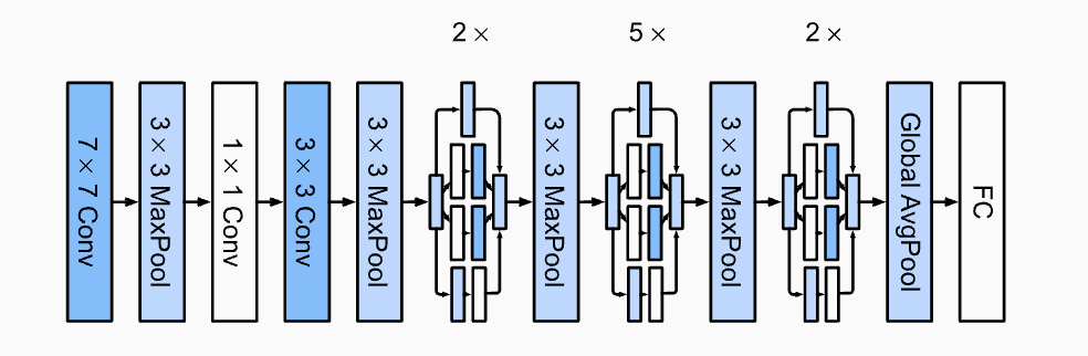
GoogLeNet

GoogLeNet designed a multi-branch structure called Inception Block

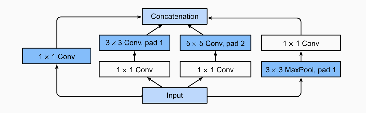
for the input, it use different size of convolutional kernels to extract new features and contact the result of all branchs in feature dimension. In order to do contatenation sucessfully, the output height and width of each branch should be the same.

The each branch in inception block keep the height and width the same as the input. While during blocks, it use pooling layer to half height and width.

Moreover, in the final layer, it use a single full connect layer simply to match the output with number of classes.

GoogLeNet structure:

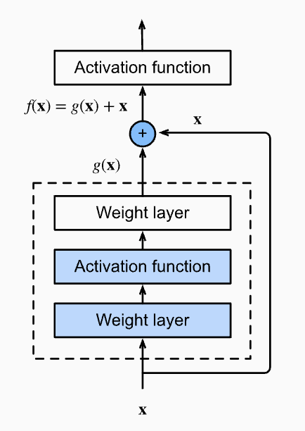
ResNet

ResNet is a net that will add input back into output for each block

In order to add input and output successfully, the number of channels, width and height should all be the same. So, normally, we will use 1x1 convolutional kernel to do some transform on the input. The resnet-18 architecture:  ## ResNeXt Block ResNeXt Block use a grouped convolution to speed up calculation of convolutional block. In a convolutional layer with out grouped convolution, if the input channel is $c_i$ and the output channel is $c_o$, the computational cost of this layer is proportional to $O(c_i \cdot c_o)$. If we use grouped convolution, we will split the input channels into $g$ groups, so, for each group, the input channel size is $\frac{c_i}{g}$, and we output $\frac{c_o}{g}$ number of channels for every group. Then we contact the outputs from all groups into $c_o$ channels. Hence, after grouped convolution, the computational cost for each group is $O(\frac{c_i}{g} \cdot \frac{c_o}{g})$, and the computational cost of the total group is $O(g \cdot \frac{c_i}{g} \cdot \frac{c_o}{g})=O(\frac{c_i \cdot c_o}{g})$. So, If the group size is $g$, then the speed is theoretically g times faster.  ## DenseNet DenseNet like ResNet, will utilize the input in each convolutional block (dense block), but instead of add the input with the output elementwisely, it concat the input and output in channel dimension.  As for the dense block, it consists of multiple convolution blocks, each using the same number of output channels. And in order to enable concatation with input and output in channel dimension, the dense block convolutional layers will keep the width and height unchanged. Since each dense block will increase the number of channels, adding too many of them will lead to an excessively complex model. A transition layer is used to control the complexity of the model. It reduces the number of channels by using a 1x1 convolution. Moreover, it halves the height and width via average pooling with a stride of 2. # Batch Normalization Batch Normalization is a technique to accelerate the convergence of deep neural network. It is defined as: $$ BN(X) = \gamma \odot \frac{x- \hat{\mu_{B}}}{\hat{\sigma_{B}}} + \beta $$ Where $\mu_{B}$ is the sample mean and $\sigma_{B}$ is the sample standard deviation of the minibatch $B$, Batch Normalization has training parameter $\gamma$ and $\beta$. After applying standardization, the resulting minibatch has zero mean and unit variance. The choice of unit variance (rather than some other magic number) is arbitrary. We recover this degree of freedom by including an elementwise scale parameter $\gamma$ and shift parameter $\beta$. Batch Normalization will be used both in training process and inference process, but during the two phases, it has different behaviors. During train phase, the mean and variance is calculated with a batch of data, meanwhile, we accumulate the mean amd variance of the whole training data with momentum. Then during inference phase, we apply the learn $\gamma$, $\beta$, and the accumulated mean and variance to calculate the output of the Batch Normalization Layer. Basically, Batch Normalization will first normalize the batch data to mean equal to 0 and variance equal to 1 for each feature, then shift the data to mean equal to $\gamma$ and variance to $\beta$. Because Batch Normalization calculates mean and variance among a batch of data, the batch size parameter has a significant influence on the Batch Normalization. Usually, Batch Normalization layer is applied after Convolutional Layer and before activation function. # Layer Normalization The difference of Layer Normalization and Batch Normalization is that Layer Norm calculate mean and variance based on a single data among all features, while Batch Normalization calculate mean and variance based on a single feature among a batch of data. Hence, Layer Normalization is not sensitive to batch size we choose. In addition, layer normalization has no learning parameters. Layer Normalization is often used in transformer for vision like ViT net. # Computer Vision ## Image Augmentation ## Fine-Tuning ## Single Shot Multibox Detection ## R-CNNS # RNN ## Raw Test into Sequence Data * Tokenize the raw text and build a vocabulary * token is the atomic(indivisible) units of text, the simplest way is to tokenize text by characters or words, but modern model use more complex way to tokenize text. * vocabulary is a map that can encode token to number can decode number back to token * then we encode the whole raw text into a sequence of number * next, we need to convert the whole sequence of number into our training/testing features and label. * we choose a time step n, we randomly choose n length of sequence of number as features and the label is the token that exact one token shift of the feature token. For example, if the text is "hello, world", and the time step we choose is 4, then a training data can be ['h', 'e', 'l', 'l'], then corresponding label data is ['e', 'l', 'l', 'o'], which means if the network sees 'h', it need to output 'e', if it sees 'e', then it should output 'l', etc. ## rnn RNN is a network with hidden state $$ \begin{align*} H_t & = \phi(X_t W_{xh} + H_{t-1} W_{hh} + b_{h}) \\ O & = H_{t} W_{ho} + b_{o} \end{align*} $$ $t$ range in $[1, \text{Number of Time Steps}]$, Nomally, we will initialize the initial hidden state $H_{0}$ with zeros.  During training steps, the feature data $X$ from dataset usually in the shape of $(batch\_size, time\_steps, vocab\_size)$ , normally will put the time_steps dimension to first, i.e. $(time\_steps, batch\_size, vocab\_size)$. After that, in every time step, we can calculate hidden states and output by batch. And for every number time_steps of data in a batch, they corresponding to their own sequence of hidden states.

Perplexity

Basically, perlexity is the exponential value of cross entropy loss. We can use perlexity to evaluate the performance of a lanuage model. During training step we still the result of cross entropy loss to calculate the gradients and update parameters. The cross entropy loss ranges in $[0, +\infty]$, so the perplexity ranges in $[1, +\infty]$.

Modern RNN

LSTM & GRU

LSTM and GRU are RNN models with more complex hidden states, they mainly design to prevent gradient exploding in training rnn.

Deep RNN

deep rnn increase the number of layers of hidden states.

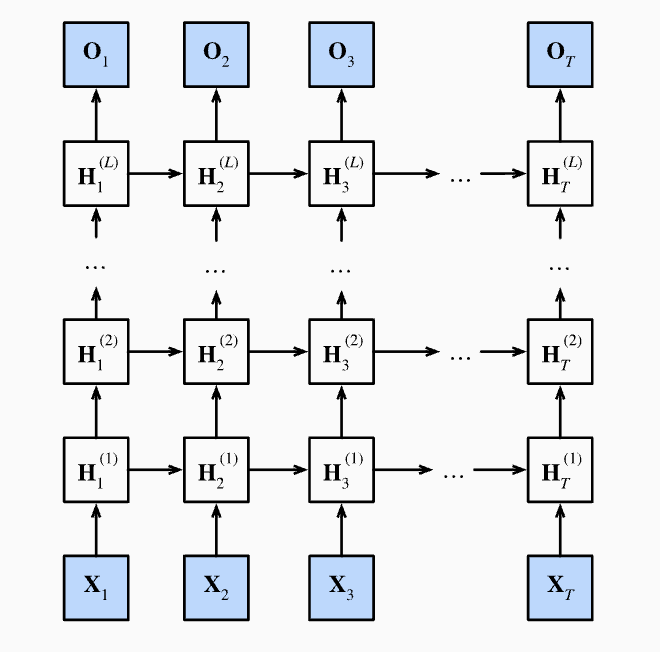
As depicted in the graph, Hidden state is computed by:

$$H_{t}^{(l)} = \phi_{l}(H_{t}^{(l-1)} W_{xh}^{(l)} + H_{t-1}^{(l)} W_{hh}^{l} + b_{h}^{(l)})$$

To use deep rnn in pytorch, we only need to simply use the num_layers parameter

nn.RNN(input_size=vocab_size, hidden_size=32, num_layers=4)
nn.GRU(input_size=vocab_size, hidden_size=32, num_layers=4)
nn.LSTM(input_size=vocab_size, hidden_size=32, num_layers=4)

Bidirectional RNN

In Bidirectional RNN, in each hidden layer, there is a hidden state calculated from $t_1$ to $t_n$ and a hidden state calculated from $t_n$ to $t_1$, after that, we concat the hidden state in horizontal direction. As a result, the final output size of hidden state is the double of each hidden state size.

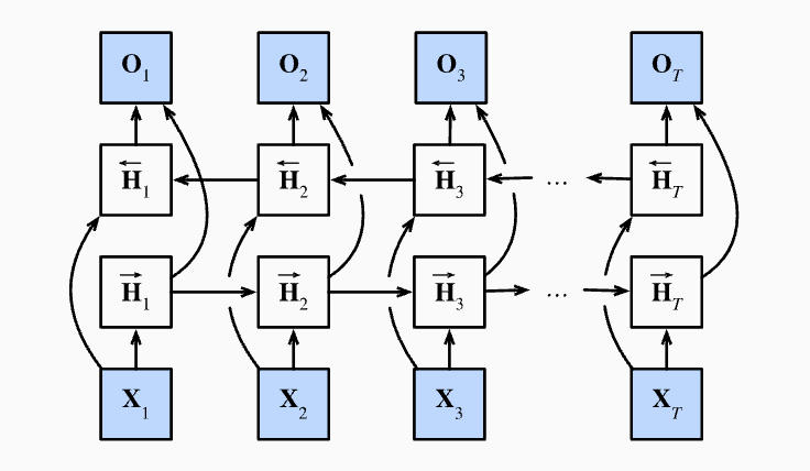
A trick to calculate hidden state from $t_n$ to $t_1$ is to reverse input $X$ to $X_t$ to $X_1$ and then do calculated like normal input, this can speed up calculate instead of use for loop from $t$ to $1$.

Bidirectional RNNs are mostly useful for sequence encoding and the estimation of observations given bidirectional context.

Bidirectional RNNs are very costly to train due to long gradient chains.

Bidirectional RNNs are not quite useful in predicting next token by given tokens, as there are only information from past was given during prediction.

Encoder-Decoder Framework

Encoder-Decoder for Machine Translation

Beam Search

Attention Mechanisms and Transformers

Queries, Keys, and Values

Reinforcement Learning

GAN

Engineering

Parameter Initialization and Management

Lazy Initialization

Compute Devices

Model Backend

Data Parallization in Multiple GPUs.