ProseMirror Guide

Introduction

There are four essential modules, which are required to do any editing at all

• prosemirror-model defines the editor’s document model, the data structure used to describe the content of the editor.

• prosemirror-state provides the data structure that describes the editor’s whole state, including the selection, and a transaction system for moving from one state to the next.

• prosemirror-view implements a user interface component that shows a given editor state as an editable element in the browser, and handles user interaction with that element.

• prosemirror-transform contains functionality for modifying documents in a way that can be recorded and replayed, which is the basis for the transactions in the state module, and which makes the undo history and collaborative editing possible.

1
2
3
4
5
6

import {schema} from "prosemirror-schema-basic"
import {EditorState} from "prosemirror-state"
import {EditorView} from "prosemirror-view"

let state = EditorState.create({schema})
let view = new EditorView(document.body, {state})

Transactions

When the user types, or otherwise interacts with the view, it generates ‘state transactions’. What that means is that it does not just modify the document in-place and implicitly update its state in that way. Instead, every change causes a transaction to be created, which describes the changes that are made to the state, and can be applied to create a new state, which is then used to update the view. By default this all happens under the cover, but you can hook into by writing plugins or configuring your view.

Plugins

Plugins are used to extend the behavior of the editor and editor state in various ways.

Command

Most editing actions are written as commands which can be bound to keys, hooked up to menus, or otherwise exposed to the user.

Content

A state’s document lives under its doc property. This is a read-only data structure, representing the document as a hierarchy of nodes, somewhat like the browser DOM. A simple document might be a "doc" node containing two "paragraph" nodes, each containing a single "text" node.

When initializing a state, you can give it an initial document to use. In that case, the schema field is optional, since the schema can be taken from the document.

1
2
3
4
5
6
7
8

import {DOMParser} from "prosemirror-model"
import {EditorState} from "prosemirror-state"
import {schema} from "prosemirror-schema-basic"

let content = document.getElementById("content")
let state = EditorState.create({
  doc: DOMParser.fromSchema(schema).parse(content)
})

Documents

structure

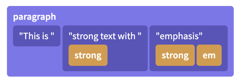
A ProseMirror document is a node, which holds a fragment containing zero or more child nodes.
This is a lot like the browser DOM, in that it is recursive and tree-shaped. But it differs from the DOM in the way it stores inline content. Whereas in ProseMirror, the inline content is modeled as a flat sequence, with the markup attached as metadata to the nodes.

Identity and persistence

In the DOM, nodes are mutable objects with an identity, which means that a node can only appear in one parent node, and that the node object is mutated when it is updated.

This has a bunch of advantages. It makes it impossible to have an editor in an invalid in-between state during an update, since the new state, with a new document, can be swapped in instantaneously. It also makes it easier to reason about documents in a somewhat mathematical way, which is really hard if your values keep changing underneath you. This helps make collaborative editing possible and allows ProseMirror to run a very efficient DOM update algorithm by comparing the last document it drew to the screen to the current document.

Data structures

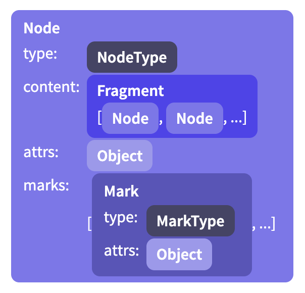
The content of a node is stored in an instance of Fragment, which holds a sequence of nodes. Even for nodes that don’t have or don’t allow content, this field is filled (with the shared empty fragment).
Some node types allow attributes, which are extra values stored with each node. For example, an image node might use these to store its alt text and the URL of the image.

In addition, inline nodes hold a set of active marks—things like emphasis or being a link—which are represented as an array of Mark instances.

1
2
3
4
5
6
7
8

import {schema} from "prosemirror-schema-basic"

// (The null arguments are where you can specify attributes, if necessary.)
let docNode = schema.node("doc", null, [
  schema.node("paragraph", null, [schema.text("One.")]),
  schema.node("horizontal_rule"),
  schema.node("paragraph", null, [schema.text("Two!")])
])

Each ProseMirror document has a schema associated with it. The schema describes the kind of nodes that may occur in the document, and the way they are nested. For example, it might say that the top-level node can contain one or more blocks, and that paragraph nodes can contain any number of inline nodes, with any marks applied to them.

Node Types

Every node in a document has a type, which represents its semantic meaning and its properties, such as the way it is rendered in the editor.

When you define a schema, you enumerate the node types that may occur within it, describing each with a spec object:

1
2
3
4
5
6
7

const trivialSchema = new Schema({
  nodes: {
    doc: {content: "paragraph+"},
    paragraph: {content: "text*"},
    text: {inline: true},
    /* ... and so on */
  }

Every schema must at least define a top-level node type (which defaults to the name "doc", but you can configure that), and a "text" type for text content.

Content Expressions

The strings in the content fields in the example schema above are called content expressions. They control what sequences of child nodes are valid for this node type.

For example "paragraph" for “one paragraph”, or "paragraph+" to express “one or more paragraphs”. Similarly, "paragraph*" means “zero or more paragraphs” and "caption?" means “zero or one caption node”. You can also use regular-expression-like ranges, such as {2} (“exactly two”) {1, 5} (“one to five”) or {2,} (“two or more”) after node names.

Such expressions can be combined to create a sequence, for example "heading paragraph+" means ‘first a heading, then one or more paragraphs’. You can also use the pipe | operator to indicate a choice between two expressions, as in "(paragraph | blockquote)+".
Some groups of element types will appear multiple times in your schema—for example you might have a concept of “block” nodes, that may appear at the top level but also nested inside of blockquotes. You can create a node group by giving your node specs a group property, and then refer to that group by its name in your expressions.

1
2
3
4
5
6
7
8

const groupSchema = new Schema({
  nodes: {
    doc: {content: "block+"},
    paragraph: {group: "block", content: "text*"},
    blockquote: {group: "block", content: "block+"},
    text: {}
  }
})

Here "block+" is equivalent to "(paragraph | blockquote)+".

It is recommended to always require at least one child node in nodes that have block content (such as "doc" and "blockquote" in the example above), because browsers will completely collapse the node when it’s empty, making it rather hard to edit.

The order in which your nodes appear in an or-expression is significant.

Marks

Marks are used to add extra styling or other information to inline content. A schema must declare all mark types it allows in its schema. Mark types are objects much like node types, used to tag mark objects and provide additional information about them.

By default, nodes with inline content allow all marks defined in the schema to be applied to their children. You can configure this with the marks property on your node spec.

1
2
3
4
5
6
7
8
9
10
11
12

const markSchema = new Schema({
  nodes: {
    doc: {content: "block+"},
    paragraph: {group: "block", content: "text*", marks: "_"},
    heading: {group: "block", content: "text*", marks: ""},
    text: {inline: true}
  },
  marks: {
    strong: {},
    em: {}
  }
})

The set of marks is interpreted as a space-separated string of mark names or mark groups—"_" acts as a wildcard, and the empty string corresponds to the empty set.

Attributes

The document schema also defines which attributes each node or mark has. If your node type requires extra node-specific information to be stored, such as the level of a heading node, that is best done with an attribute.

1
2
3
4

heading: {
    content: "text*",
    attrs: {level: {default: 1}}
  }

In this schema, every instance of the heading node will have a level attribute under .attrs.level. If it isn’t specified when the node is created, it will default to 1.
When you don’t give a default value for an attribute, an error will be raised when you attempt to create such a node without specifying that attribute.

Serialization and Parsing

In order to be able to edit them in the browser, it must be possible to represent document nodes in the browser DOM. The easiest way to do that is to include information about each node’s DOM representation in the schema using the toDOM field in the node spec.

Documents also come with a built-in JSON serialization format. You can call toJSON on them to get an object that can safely be passed to JSON.stringify, and schema objects have a nodeFromJSON method that can parse this representation back into a document.

Extending a schema

The schema-list module exports a convenience method to add the nodes exported by those modules to a nodeset.

Document transformations

Transforms are central to the way ProseMirror works. They form the basis for transactions, and are what makes history tracking and collaborative editing possible.

Steps

Updates to documents are decomposed into steps that describe an update. You usually don’t need to work with these directly, but it is useful to know how they work. Examples of steps are ReplaceStep to replace a piece of a document, or AddMarkStep to add a mark to a given range.

applying a step can fail, for example if you try to delete just the opening token of a node, that would leave the tokens unbalanced, which isn’t a meaningful thing you can do. This is why apply returns a result object, which holds either a new document, or an error message. You’ll usually want to let helper functions generate your steps for you, so that you don’t have to worry about the details.

Transforms

An editing action may produce one or more steps. The most convenient way to work with a sequence of steps is to create a Transform object (or, if you’re working with a full editor state, a Transaction, which is a subclass of Transform).

Rebasing

When doing more complicated things with steps and position maps, for example to implement your own change tracking, or to integrate some feature with collaborative editing, you might run into the need to rebase steps.

You might not want to bother studying this until you are sure you need it.

The editor state

What makes up the state of an editor? You have your document, of course. And also the current selection. And there needs to be a way to store the fact that the current set of marks has changed, when you for example disable or enable a mark but haven’t started typing with that mark yet.
Those are the three main components of a ProseMirror state, and exist on state objects as doc, selection, and storedMarks.

Selection

Selections are represented by instances of (subclasses of) the Selection class. Like documents and other state-related values, they are immutable—to change the selection, you create a new selection object and a new state to hold it.

Selections have, at the very least, a start (.from) and an end (.to), as positions pointing into the current document. Many selection types also distinguish between the anchor (unmoveable) and head (moveable) side of the selection, so those are also required to exist on every selection object.

Transactions

State updates happen by applying a transaction to an existing state, producing a new state. Conceptually, they happen in a single shot: given the old state and the transaction, a new value is computed for each component of the state, and those are put together in a new state value.
Transaction is a subclass of Transform, and inherits the way it builds up a new document by applying steps to an initial document. In addition to this, transactions track selection and other state-related components, and get some selection-related convenience methods such as replaceSelection.

Plugin

When creating a new state, you can provide an array of plugins to use. These will be stored in the state and any state that is derived from it, and can influence both the way transactions are applied and the way an editor based on this state behaves.

Plugins are instances of the Plugin class, and can model a wide variety of features. The simplest ones just add some props to the editor view, for example to respond to certain events. More complicated ones might add new state to the editor and update it based on transactions.

When creating a plugin, you pass it an object specifying its behavior:

1
2
3
4
5
6
7
8

let myPlugin = new Plugin({
  props: {
    handleKeyDown(view, event) {
      console.log("A key was pressed!")
      return false // We did not handle this
    }
  }
})

The view componet

A ProseMirror editor view is a user interface component that displays an editor state to the user, and allows them to perform editing actions on it.

The definition of editing actions used by the core view component is rather narrow—it handles direct interaction with the editing surface, such as typing, clicking, copying, pasting, and dragging, but not much beyond that. This means that things like displaying a menu, or even providing a full set of key bindings, lie outside of the responsibility of the core view component, and have to be arranged through plugins.

Editable DOM

Browsers allow us to specify that some parts of the DOM are editable, which has the effect of allowing focus and a selection in them, and making it possible to type into them. The view creates a DOM representation of its document (using your schema’s toDOM methods by default), and makes it editable. When the editable element is focused, ProseMirror makes sure that the DOM selection corresponds to the selection in the editor state.

most cursor-motion related keys and mouse actions are handled by the browser, after which ProseMirror checks what kind of text selection the current DOM selection would correspond to. If that selection is different from the current selection, a transaction that updates the selection is dispatched.

Even typing is usually left to the browser, because interfering with that tends to break spell-checking, autocapitalizing on some mobile interfaces, and other native features. When the browser updates the DOM, the editor notices, re-parses the changed part of the document, and translates the difference into a transaction.

Data flow

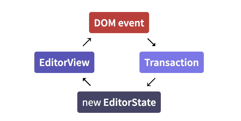
Efficient updating

One way to implement updateState would be to simply redraw the document every time it is called. But for large documents, that would be really slow.
Since, at the time of updating, the view has access to both the old document and the new, it can compare them, and leave the parts of the DOM that correspond to unchanged nodes alone. ProseMirror does this, allowing it to do very little work for typical updates.

Commands

In ProseMirror jargon, a command is a function that implements an editing action, which the user can perform by pressing some key combination or interacting with the menu.

The prosemirror-commands module provides a number of editing commands, from simple ones such as a variant of the deleteSelection command, to rather complicated ones such as joinBackward, which implements the block-joining behavior that should happen when you press backspace at the start of a textblock. It also comes with a basic keymap that binds a number of schema-agnostic commands to the keys that are usually used for them.

When possible, different behavior, even when usually bound to a single key, is put in different commands. The utility function chainCommands can be used to combine a number of commands—they will be tried one after the other until one return true.

Collaborative editing

Real-time collaborative editing allows multiple people to edit the same document at the same time. Changes they make are applied immediately to their local document, and then sent to peers, which merge in these changes automatically.

Algorithm

ProseMirror’s collaborative editing system employs a central authority which determines in which order changes are applied. If two editors make changes concurrently, they will both go to this authority with their changes. The authority will accept the changes from one of them, and broadcast these changes to all editors. The other’s changes will not be accepted, and when that editor receives new changes from the server, it’ll have to rebase its local changes on top of those from the other editor, and try to submit them again.

VPC

Internet Gateway

internet gateway is responsible for connection between resources under vpc with public ips and the internet.

Subnet

differnet Subnets can associate different Route Tables, if the subnet associated a route table with a destination to Internet Gateway, this subnet can be considered as public subnet.

NAT

NAT is responsible for connection between resources under vpc only with private ips and the internet. It’s a one way connection, only the private resource can reach the external internet, the external internet can not reach the private resource with NAT. The NAT need to bind a Elastic IP, which is a public IP, hence, the NAT need to be defined in a public subnet (the subnet has a route table item to Internet Gateway).

Load balancer

Load balancer is like the reverse version of NAT, it support external network traffic to going into internal public and private resources if it’s a internet facing load balancer. Normally internet facing load balancer will have public IP address, those address can be seem in ENI(Elastic Network Interfaces).

Load balancer essential is a nginx, it can create routing rules to different target group and add ssl certificate

Preliminaries

Data Preprocessing

In real life data, usually there will be missing values. Depending upon the context, missing values might be handled either via imputation or deletion.

• Imputation: replaces missing values with estimates of their values

• Deletion: simply discards either those rows or those columns that contain missing values.

Linear Model

Linear Regression

Leanr Regression Model can be represented as $\hat{y} = Xw + b$, where $X$ is in the shape of $[\text{batch_size}, \text{num_features}]$, $w$ is in the shape of $[\text{num_features}, 1]$, b is a scale value. Correspondingly, $\hat{y}$ is in the shape of $[\text{batch_size}, 1]$

Linear Regression Model usually use Mean Square Loss as loss function

LeNet

The first Deep CNN.

1
2
3
4
5
6
7
8
9
10
11
12
13
14
15
16
17
18
19

self.net = nn.Sequential(
            nn.LazyConv2d(6, kernel_size=5, padding=2), 
            nn.Sigmoid(),
            nn.AvgPool2d(kernel_size=2, stride=2),

            nn.Conv2d(6, 16, kernel_size=5), 
            nn.Sigmoid(),
            nn.AvgPool2d(kernel_size=2, stride=2),

            nn.Flatten(),

            nn.LazyLinear(120),
            nn.Sigmoid(),

            nn.Linear(120, 84),
            nn.Sigmoid(),

            nn.Linear(84, num_classes)
        )

Modern CNN

AlexNet

AlexNet is basically a bigger and deep version of LeNet.

1
2
3
4
5
6
7
8
9
10
11
12
13
14
15
16
17
18
19
20
21
22
23
24
25
26
27
28
29
30
31

self.net = nn.Sequential(
            nn.LazyConv2d(96, kernel_size=11, stride=4, padding=1),
            nn.ReLU(),
            nn.MaxPool2d(3, stride=2),

            nn.Conv2d(96, 256, kernel_size=5, padding=2),
            nn.ReLU(),
            nn.MaxPool2d(3, stride=2),

            nn.Conv2d(256, 384, kernel_size=3, padding=1),
            nn.ReLU(),

            nn.Conv2d(384, 384, kernel_size=3, padding=1),
            nn.ReLU(),

            nn.Conv2d(384, 256, kernel_size=3, padding=1),
            nn.ReLU(),
            nn.MaxPool2d(3, stride=2),

            nn.Flatten(),

            nn.LazyLinear(4096),
            nn.ReLU(),
            nn.Dropout(0.5),

            nn.Linear(4096, 4096),
            nn.ReLU(),
            nn.Dropout(0.5),

            nn.Linear(4096, num_classes)
        )

VGG

VGG provide a general template to design convolutional nerual network which is use net blocks. In VGG, the layers in a block are basic Conv Layer, Activation Layer and Pooling Layer

block code

1
2
3
4
5
6
7
8
9
10
11
12
13

def vgg_block(num_convs, out_channels):
    """
    @param num_convs: number of convolutional layers
    @param out_channels: number of output channels, the channel num will be 
        changed immediately in the first conv layer
    """
    layers = []
    for _ in range(num_convs):
        layers.append(nn.LazyConv2d(out_channels, kernel_size=3, padding=1))
        layers.append(nn.ReLU())

    layers.append(nn.MaxPool2d(2, stride=2))
    return nn.Sequential(*layers)

net structure

1
2
3
4
5
6
7
8
9
10
11
12
13
14
15
16
17
18
19

conv_blocks = []
for (num_convs, out_channels) in arch:
    conv_blocks.append(vgg_block(num_convs, out_channels))

    self.net = nn.Sequential(
        *conv_blocks,

        nn.Flatten(),

        nn.LazyLinear(4096),
        nn.ReLU(),
        nn.Dropout(0.5),

        nn.Linear(4096, 4096),
        nn.ReLU(),
        nn.Dropout(0.5),

        nn.Linear(4096, num_classes)
    )

NiN(Network in Network)

NiN Replaces the Full Connect Layers in CNN with Global Avg Pool, which significant reduces training parameters.

NiN block:

1
2
3
4
5
6
7
8
9
10
11
12

def nin_block(out_channels, kernel_size, stride, padding):
    block = nn.Sequential(
        nn.LazyConv2d(out_channels, kernel_size=kernel_size, stride=stride, padding=padding),
        nn.ReLU(),

        nn.Conv2d(out_channels, out_channels, kernel_size=1),
        nn.ReLU(),

        nn.Conv2d(out_channels, out_channels, kernel_size=1),
        nn.ReLU()
    )
    return block

NiN net structure

1
2
3
4
5
6
7
8
9
10
11
12
13
14
15
16
17
18
19
20
21

self.net = nn.Sequential(
            nin_block(96, kernel_size=11, stride=4, padding=0),
            nn.MaxPool2d(3, stride=2),

            nin_block(256, kernel_size=5, stride=1, padding=2),
            nn.MaxPool2d(3, stride=2),

            nin_block(384, kernel_size=3, stride=1, padding=1),
            nn.MaxPool2d(3, stride=2),

            # nn.Dropout in cnn will random drop some pixel at every channel
            # nn.dropout2d in cnn will drop some entire channels
            nn.Dropout(0.5),

            # import here: we reduce channels to number of classes
            nin_block(num_classes, kernel_size=3, stride=1, padding=1),
            # adaptive pool will make the result height and width to the target size
            nn.AdaptiveAvgPool2d((1, 1)),

            nn.Flatten()
        )

GoogLeNet

GoogLeNet designed a multi-branch structure called Inception Block

for the input, it use different size of convolutional kernels to extract new features and contact the result of all branchs in feature dimension. In order to do contatenation sucessfully, the output height and width of each branch should be the same.

The each branch in inception block keep the height and width the same as the input. While during blocks, it use pooling layer to half height and width.

Moreover, in the final layer, it use a single full connect layer simply to match the output with number of classes.

GoogLeNet structure:

ResNet

ResNet is a net that will add input back into output for each block

Perplexity

Basically, perlexity is the exponential value of cross entropy loss. We can use perlexity to evaluate the performance of a lanuage model. During training step we still the result of cross entropy loss to calculate the gradients and update parameters. The cross entropy loss ranges in $[0, +\infty]$, so the perplexity ranges in $[1, +\infty]$.

Modern RNN

LSTM & GRU

LSTM and GRU are RNN models with more complex hidden states, they mainly design to prevent gradient exploding in training rnn.

Deep RNN

deep rnn increase the number of layers of hidden states.

As depicted in the graph, Hidden state is computed by:

To use deep rnn in pytorch, we only need to simply use the num_layers parameter

1
2
3

nn.RNN(input_size=vocab_size, hidden_size=32, num_layers=4)
nn.GRU(input_size=vocab_size, hidden_size=32, num_layers=4)
nn.LSTM(input_size=vocab_size, hidden_size=32, num_layers=4)

Bidirectional RNN

In Bidirectional RNN, in each hidden layer, there is a hidden state calculated from $t_1$ to $t_n$ and a hidden state calculated from $t_n$ to $t_1$, after that, we concat the hidden state in horizontal direction. As a result, the final output size of hidden state is the double of each hidden state size.

A trick to calculate hidden state from $t_n$ to $t_1$ is to reverse input $X$ to $X_t$ to $X_1$ and then do calculated like normal input, this can speed up calculate instead of use for loop from $t$ to $1$.

Bidirectional RNNs are mostly useful for sequence encoding and the estimation of observations given bidirectional context.

Bidirectional RNNs are very costly to train due to long gradient chains.

Bidirectional RNNs are not quite useful in predicting next token by given tokens, as there are only information from past was given during prediction.

Encoder-Decoder Framework

Encoder-Decoder for Machine Translation

Beam Search

Attention Mechanisms and Transformers

Queries, Keys, and Values

Reinforcement Learning

GAN

Engineering

Parameter Initialization and Management

Lazy Initialization

Compute Devices

Model Backend

Data Parallization in Multiple GPUs.

Markov Models

Markov assumption states that the probability of the current state depends only on a finite series of previous states. As a special case, this assumption gives rise to the Markov chain representation, asserting that future state predictions are conditionally independent of the past given the present state-$P(Xt | X{t-1})$

Hidden Markov Models

In hidden markov models, our agent usually don’t have a information about the state, , instead, our agents gather observations over time.

A Hidden Markov Model consists of three fundamental components: the initial distribution $P(X1)$, transition probabilities denoted by $P(Xt | X{t-1})$, and observation probabilities $P(O_t | X_t)$. Additionally, HMMs operate under two critical Markov assumptions:

1. The future states of the system depend solely on the present state, encapsulated by the transition probabilities $P(Xt | X{t-1})$.

2. The observation at a particular time step depend solely on the current state, encapsulated by the transition probabilities $P(O_t | X_t)$.

Compute the probability of an observation sequence

If we know the hidden state sequence, then the computation of the probability is straightforward.

To compute $P(s_1 | s_0)$ in the above equation (the probability of being in a specific hidden state at the first time step), we often simply resort to using the stationary distribution of the Markov chain defined over the hidden states.

If we do not know the hidden state sequence, only know the observation sequence, then, in this scenario, we need to account for all possible hidden-state sequences, and sum over their joint probabilities with the observation sequence.

However, if we do bruteforcely, for an HMM with $N$ hidden states and an observation sequence of $T$ observations, there are $N^T$ possible hidden sequences, which is unacceptable. To solve this problem, we can exploit the fact that the probability of the observation sequence up to time $t$ can be computed using the probability of the observation sequence up to time $t-1$. This is done by summing over the probabilities of all possible hidden-state sequences at time:

Then, we have

Having the recurrance, we can use dynamic programming to solve this problem with a $O(N^2 T)$ time complexity. Still, at $t=1$, we use stationary distribution to compute $P(O_{0 \to 1} | (s_1 = s_i) = P(s_i)P(o_1 |s_i)$.

Compute the most likely state sequence base on observation sequence

We use Viterbi algorithm to solve this. Very much like the dp program in previous part:

The final probability of the most likely hidden state sequence $S$ after $T$ time-steps is then given by

Then

Markov Decision Process(MDP)

When an action taken from a state is no longer guaranteed to lead to a specific successor state. Instead, we now consider the scenario where there is a probability associated with each action leading our agent from one state to another.

For example from state $S_1$, the agent takes action $a$ , but may end up in state $S_2$ with probability of $p$ and $S_3$ with probability of $1-p$ . This stochastic system can be formally represented as a markov decision process(MDP).

For MDP, we have those info:

• State Space $S$ : the set of all possible states that the system can be in.

• Action Space $A$ : the set of all possible actions, if there is no actions can be taken from states, those states are therefore terminal or end states in the MDP.

• Transition Probabilities $T$ : a the probabilities of transitioning from one state to another given a specific action, notated as $T(s, a, s’)$, where $s$ is the source state, $a$ is the action and $s’$ is the target/successor state.

• Rewards $R$ : a numerical reward associated with each transition. In general, $R(s, a, s’)$ should be thought of as the reward of reaching state $s’$ from state $s$ using action $a$.

• Discount Factor $\gamma$ : accounts for the discounting of future rewards in decision-making. It ensures that immediate rewards are valued more than future rewards. Discounting rewards in general prevents the agent from choosing actions that may lead to infinite rewards (cyclical paths).

• Policy $\pi$ : a policy is defined as a mapping from states to actions. In other words, a policy defines a choice of one action for every state in MDP. Note that a policy does not concern itself with the transition probabilities or rewards, but only with the actions to be taken in each state. It also says nothing about a specific path the agent might end up taking as a result of the chosen actions. Different policies, therefore, may lead to different cumulative rewards on average. The goal of the agent in an MDP is to find the policy that maximizes the expected cumulative reward over time. This is known as the optimal policy. Here is a policy example: ${s_0: a_0, s_1: a_1, \dots, s_n:a_n}$, this policy says that: in state $s_0$, always take action $a_0$, in state $s_1$, always take action $a_1$, and so on.

Evaluation policies

In order to find the best policy for our agent, we must be able to compare two or more given policies quantitatively. Under any one policy, even every time the agent is in a state, it takes the same action, the agent may end up in a different state each time (based on the values in Transition Probabilities $T$), so the outcome of the policy may vary, This is why we need to evaluate policies in terms of their expected cumulative rewards rather than what happens in any one specific sample.

A single actual path taken by the agent as a result of following a policy is called an episode. We define the Reward of an episode as the discounted sum of rewards along the path. Given the episode $E = (s_0, a_0, r_0, s_1, a_1, r_1, \dots, s_n, a_n, r_n)$, the Reward of the episode is given by:

where $r_t$ is the reward at time , and $\gamma$ is the discount factor. The expected Reward of a policy $\pi$ is then given by the expected value of the Reward of the episodes generated by the policy. Given a series of episodes, the expected value is simply the average of the utilities obtained in each episode; i.e., given a set of episodes $E_1, E_2, \dots, E_n$, the expected utility of the policy is given by:

By the definition above, we can deduce to the Bellman equation:

When $a=\pi(s)$, then $Q{\pi}(s, a)=V{\pi}(s)$, and the value of the state under the policy $\pi$ is then given by:

While in certain situations, the above equations may yield a closed-form solution for the value of a state under a policy, in general, we need to solve a system of linear equations to find the value of each state under the policy. This is done using a dynamic programming algorithm that iteratively computes the value of each state under the policy until the values converge. This algorithm is called the Policy Evaluation algorithm, and works as follows. We re-write the above equation to use previous estimates of $V{\pi}(s)$ to compute new estimates of $V{\pi}(s)$ as follows:

where $V_{\pi}^{(t)}$ is the estimate of the value of state $s$ under policy $\pi$ at iteration $t$. We start with an initial guess for the value of each state (usually set to 0), and then iteratively update the value of each state using the above equation until the values converge.

Find the Best Policy

Now that we have a way to evaluate the value of each state under a policy, we can use this information to find the best policy. The best policy is the one that maximizes the value of each state.

Given the value of each state $V{\pi}(s)$ under some policy $\pi$, we can find the best action for each state by simply taking the action maximizes the expected value, i.e. $\argmax{a} Q_{\pi}(s, a)$. This is known as the greedy policy.

We can use the policy evaluation algorithm to evaluate one policy, and then find the best action for each state to form a new policy. We can then evaluate this new policy and form next new policy, and so on, until the policy converges. This is known as the policy iteration algorithm. The step of policy iteration algorithm:

• Initialize an guess for the value of each state $V(s)$ (usually set to 0)

• Then we caculate Q-value of each possible action under a state $Q(s, a)$

• After that, we can decide each state the currrent optimal action and form a new policy $\pi_{opt}$

• Assign the maximum $Q(s, a)$ to the new $V(s)$

• Then redo the process until the policy converges.

there is one key difference between policy evaluation alogrithm and policy iteration alogrithm: instead of using a fixed policy $\pi$, we use the greedy policy at each iteration such that the chosen action maximizes the expected value.

Partially Observable MDPS

In the previous discussion about MDP, agent knows precisely which state in the state-space it is currently in. However, in many real-life implementations of autonomous agents, the agent does not have a global view of the world, but must instead rely on observations of its immediate surroundings. Using these observations, the agent may then compute how likely it is to be in every possible state in the state space. Such scenarios can be modeled using the Partially Observable MDP (or POMDP) framework.

A POMDP need 2 more elements than MDP:

• Observation Space $O$: the set of all possible observations that the agent can make.

• Observation Probabilities $\Omega$ : a function that gives the probability of making an observation given a specific state

As in the MDP, the agent’s goal in a POMDP is to find the policy that maximizes the expected cumulative reward over time.

Now, given an observation, the agent must update its belief about which state it is actually in, since the agent does not know this for sure. The belief state is defined as a probability distribution over the state space, representing the agent’s likelihood of being in each state in the state-space.

Instead of moving from state $s$ to $s’$ in MDP, in a POMDP, the agent transitions between belief states, say $b$ to $b’$ as the result of an action .

Given an observation, we need to calcuate the probability of being one state, i.e. $P(s|o)$. Luckily, Bayes’ theorem allows us to invert this dependency, and compute the probability as follows:

where $P(o|s)$ is the probability of making the observation $o$ given the state $s$ - this is nothing but $\Omega(o, s)$, $P(s)$ is the prior probability of being in state $s$, and $P(o)$ is the probability of making the observation $o$ from any state, and is given by:

In practice, we can usually ignore the denominator, since it is the same for all states in the equation for $P(s|o)$. Therefore, we can compute the belief state as

where $b(s)$ is the probability of being in state $s$ given the observation $o$, i.e. $P(s|o)$.

We can now begin to reason about the transition between belief states for POMDPs, instead of the transition model between states in standard MDPs. First, let us compute the belief state update resulting from this specific action and observation, and we will then discuss the belief state transition in general. The belief state update is given by:

where $b^{(t)}(s’)$ is the probability of being in state $s’$ after taking action $a$ and making observation $o$, and $b^{(t-1)}(s)$ is the last-known probability of being in state $s$ before taking action. There are a few key things to keep in mind here:

• First, note that we update the probability of being in every target cell $s’$, summing over all origin state $s$ from where the action $a$ could have brought us to $s’$. This is opposite to the MDP Bellman equation, where we update the value of every origin state $s$, summing over all target states $s’$ under the action $a$.

• Second, just like the Bellman updates, the above belief-state update is calculated for every state in the state-space, considering each as a target state under the action $a$.

• Third, result ofactions may be stochastic, therefore we still have a notion of an action taking the agent to a different state.

Now we give previous belief state, an action and an observation after that action, we can compute the new belief state. Next, we need to estimate $T(b, a, b’)$, the probability of transitioning to one specific belief state from a previous one, given an action, accounting for all possible observations as a result of that action. We must keep in mind that unlike the number of states in an MDP, the number of belief states in a POMDP is infinite, since every probability distribution over the state-space is a valid belief state. However, given any one belief state, if we take an action and make an observation, we can only end up in one new belief state.

Reinforcement Learning

As our final layer of complexity, imagine a situation where neither the transition probabilities nor the rewards are known a priori. The action space is assumed to be fully known, and the state space may or may not be fully known. In such environments, we deploy a class of algorithms known collectively as reinforcement learning (RL), where the agent learns to make decisions through interactions with the environment. The agent may choose to infer or estimate the underlying mechanics of the world such as $T(s, a, s’)$ and $R(s, a, s’)$, or directly try to optimize the value function in search of an optimal policy.

Model Based Monte Carlo (MBMC)

we assume an underlying MDP, and use the episodes data solely to infer the model’s parameters(transition probabilities and rewards). Once we have an MDP, evaluating a given policy, or computing the optimal policy proceeds exactly as we did before. However, this approach may have a few drawbacks:

• MBMC approaches use data-based estimates to construct a fixed model of the environmentOnce this model is constructed, it is typically not updated

• The second drawback is that policy evaluation and optimal policy estimation for a given MDP is computationally expensive. To compute optimal policies, we must consider all possible actions from all states, running a large number of updates for each legal state-action pair until the values converge.

Model Free Monte Carlo (MFMC)

we use the data from the environment to directly estimate Q-values, without first constructing the underlying MDP.

Q-Learning

Q-Learning is an off-policy value-based method that uses a TD approach to train its action-value function

• First we initialize for All State-Action Value (or State Value) with 0

• We use Epsilon($\epsilon$)-Greedy Policy to choose our action

  • each step with $\epsilon$ probability to choose random action

  • with $1 - \epsilon$ probabilty to choose the optimal action

  • initially, $\epsilon$ is 1, and after some time steps, it will drop to some smaller value

• Then, we update our State-Action Value table (or State Value table) for each $(S, A, R,S’)$ pairs

  $$\begin{gather*} Q_{new}(S, A) \gets V_{old}(S, A) + lr \times [R + \gamma \times max(Q_{old}(S', A)) - Q_{old}(S, A)] \\ \text{or} \\ V_{new}(S) \gets V_{old(S)} + lr \times [R + \gamma \times V_{old}(S') - V_{old}(S)] \end{gather*}$$

Explain for the word Off-policy: using a different policy for acting and updating. For instance, with Q-Learning, the epsilon-greedy policy (acting policy), is different from the greedy policy that is used to select the best next-state action value to update our Q-value (updating policy).

While On-policy: using the same policy for acting and updating. For instance, with Sarsa, another value-based algorithm, the epsilon-greedy policy selects the next state-action pair, not a greedy policy.

Deep Q-Learning

Q-Learning worked well with small state space environments, if the states and actions spaces are not small enough to be represented efficiently by arrays and tables, Q-Learning Cannot solve those problem efficiently.

Instead of using a Q-table, Deep Q-Learning uses a Neural Network that takes a state as input and approximates Q-values for each action based on that state.

in Deep Q-Learning, we create a loss function that compares our Q-value prediction and the Q-target and uses gradient descent to update the weights of our Deep Q-Network to approximate our Q-values better.

The Deep Q-Learning training algorithm has two phases:

• Sampling: we perform actions and store the observed experience tuples in a replay memory.
• Training: Select a small batch of tuples randomly and learn from this batch using a gradient descent update step.

What

Batch normalization is applied to individual layers, or optionally, to all of them: In each training iteration, we first normalize the inputs (of batch normalization) by subtracting their mean and dividing by their standard deviation, where both are estimated based on the statistics of the current minibatch.

Next, we apply a scale coefficient and an offset to recover the lost degrees of freedom.

Convolutional Layers

Similarly, with convolutional layers, we can apply batch normalization after the convolution but before the nonlinear activation function. The key difference from batch normalization in fully connected layers is that we apply the operation on a per-channel basis across all locations. In other word, batch normalization is applied in the demension of channels, channels is kinda like the features that in the full connected layer.

Assume that our minibatches contain $m$ examples and that for each channel, the output of the convolution has height $p$ and width $q$. For convolutional layers, we carry out each batch normalization over the $m \cdot p \cdot q$ elements per output channel simultaneously. Each channel has its own scale $\gamma$ and shift $\beta$ parameters.

Layer Normalization

Note that in the context of convolutions the batch normalization is well defined even for minibatches of size 1: after all, we have all the locations across an image to average. Consequently, mean and variance are well defined, even if it is just within a single observation. This consideration led to introduce the notion of layer normalization. It works just like a batch norm, only that it is applied to one observation at a time.

For an n-dimensional vector $x$, layer norms are given by

layer normalization does not depend on the minibatch size. It is also independent of whether we are in training or test regime.

Conclusion: difference between batch normalization and layer normalization

What Can Batch normalization achieve

Bacth normalization can speed up convergence, so that we can change learning rate to a bigger value

Norms and Weight Decay

We can always mitigate overfitting by collecting more training data. However, that can be costly, time consuming, or entirely out of our control, making it impossible in the short run.

Rather than directly manipulating the number of parameters, weight decay, operates by restricting the values that the parameters can take. weight decay might be the most widely used technique for regularizing parametric machine learning models.

and the updation for w in stochastic gradient descent with this loss function will be:

every literation, we will shrink w by $lr \times \lambda$ first, that’s why this method is called weight decay.

为什么Weight Decay可以一定程度上缓解过拟合

因为在实际中，用于机器学习的数据是有噪声的，这些噪声会导致模型无法真正学习到最优的解，一般会和最优解有偏差，而且，可以证明，当噪声越大，学习到的$w$就会越大。这时可以通过weight decay调整$\lambda$的值来讲学习到的解拉近到真正最优解，如果$\lambda$过小，拉近之后的解仍然会离真正的最优解一定距离，如果$\lambda$过大，就会导致从另外一个方向远离真正最优解。

Introduction To Environment

clearColor

The ‘clearColor’ property on the scene object is the most rudimentary of environment properties/adjustments. Simply stated, this is how you change the background color of the scene. Here is how it is done:

1

scene.clearColor = new BABYLON.Color3(0.5, 0.8, 0.5);

This color and property is not used in any calculations for the final colors of mesh, materials, textures, or anything else. It is simply the background color of the scene. Easy.

ambientColor

1

scene.ambientColor = new BABYLON.Color3(0.3, 0.3, 0.3);

Mainly, it is used in conjunction with a mesh’s StandardMaterial.ambientColor to determine a FINAL ambientColor for the mesh material.

When there is no scene.ambientColor, then StandardMaterial.ambientColor and StandardMaterial.ambientTexture will appear to do nothing.

Set a scene.ambientColor of some value, StandardMaterial.ambientColor/StandardMaterial.ambientTexture will become active on meshes where you have applied such.

By default, scene.ambientColor is set to Color3(0, 0, 0), which means there is no scene.ambientColor.

Fog

Fog is quite an advanced effect, but fog in Babylon.js has been simplified to the maximum. It’s now very easy to add fog to your scenes. First, we define the fog mode like this:

1

scene.fogMode = BABYLON.Scene.FOGMODE_EXP;

• BABYLON.Scene.FOGMODE_NONE - default one, fog is deactivated.
• BABYLON.Scene.FOGMODE_EXP - the fog density is following an exponential function.
• BABYLON.Scene.FOGMODE_EXP2 - same that above but faster.
• BABYLON.Scene.FOGMODE_LINEAR - the fog density is following a linear function.

If you choose the EXP, or EXP2 mode, then you can define the density option (default is 0.1):

1

scene.fogDensity = 0.01;

if you choose LINEAR mode, then you can define where fog starts and where fog ends:

1
2

scene.fogStart = 20.0;
scene.fogEnd = 60.0;

Finally, whatever the mode, you can specify the color of the fog (default is BABYLON.Color3(0.2, 0.2, 0.3)):

1

scene.fogColor = new BABYLON.Color3(0.9, 0.9, 0.85);

Skyboxes

In Babylon.js, skyboxes typically use CubeTexture on a large cube.

The CubeTexture constructor takes a base URL and (by default) appends “_px.jpg”, “_nx.jpg”, “_py.jpg”, “_ny.jpg”, “_pz.jpg” and “_nz.jpg” to load the +x, -x, +y, -y, +z, and -z facing sides of the cube. (These suffixes may be customized if needed.)

CubeTexture images need to be .jpg format (unless the suffixes are customized) and square. For efficiency, use a power of 2 size, like 1024x1024.

Manual creation

1
2
3
4

const skybox = BABYLON.MeshBuilder.CreateBox("skyBox", { size: 100.0 }, scene);
const skyboxMaterial = new BABYLON.StandardMaterial("skyBox", scene);
skyboxMaterial.backFaceCulling = false;
skybox.material = skyboxMaterial;

Next, we set the infiniteDistance property. This makes the skybox follow our camera’s position.

1

skybox.infiniteDistance = true;

Now we must remove all light reflections on our box (the sun doesn’t reflect on the sky!):

1

skyboxMaterial.disableLighting = true;

Next, we apply our special sky texture to it. This texture must have been prepared to be a skybox, in a dedicated directory, named “skybox” in our example:

1
2

skyboxMaterial.reflectionTexture = new BABYLON.CubeTexture("textures/skybox", scene);
skyboxMaterial.reflectionTexture.coordinatesMode = BABYLON.Texture.SKYBOX_MODE;

In that /skybox directory, we must find 6 sky textures, one for each face of our box. Each image must be named per the corresponding face: “skybox_nx.jpg” (left), “skybox_ny.jpg” (down), “skybox_nz.jpg” (back), “skybox_px.jpg” (right), “skybox_py.jpg” (up), “skybox_pz.jpg” (front). The “_nx.jpg” is added to your path.

You can also use dds files to specify your skybox. These special files can contain all information required to setup a cube texture:

1

skyboxMaterial.reflectionTexture = new BABYLON.CubeTexture("/assets/textures/SpecularHDR.dds", scene);

Final note, if you want your skybox to render behind everything else, set the skybox’s renderingGroupId to 0, and every other renderable object’s renderingGroupId greater than zero

1
2
3
4

skybox.renderingGroupId = 0;

// Some other mesh
myMesh.renderingGroupId = 1;

Automatic creation

1
2

envTexture = new BABYLON.CubeTexture("/assets/textures/SpecularHDR.dds", scene);
scene.createDefaultSkybox(envTexture, true/*use a PBRMaterial*/, 1000);

Background Materials

The background material is fully unlit (which means it can still show color even there is no light created in the scene) but can still receive shadows or be subject to image processing information. This makes it the best fit to use as a skybox or the material of ground.

1

let backgroundMaterial = new BABYLON.BackgroundMaterial("backgroundMaterial", scene);

Diffuse

The diffuse part is used to simply give a color to the mesh.

1

backgroundMaterial.diffuseTexture = new BABYLON.Texture("textures/grass.jpg", scene);

Shadows

The material is able to receive shadows despite being unlit. This is actually one of its strength making it really attractive for grounds. If you want to dim the amount of shadows, you can use the dedicated properties:

1

backgroundMaterial.shadowLevel = 0.4;

Starting from Babylonjs v4.2, there’s also a new shadowOnly property that only renders shadow, making the material behave like the ShadowOnlyMaterial material but without the single light restriction.

When shadowOnly = true, you can use primaryColor to tint the shadow color and alpha to make the shadows more or less strong

1
2
3
4
5

let backgroundMaterial = new BABYLON.BackgroundMaterial("backgroundMaterial", scene);

backgroundMaterial.primaryColor = new BABYLON.Color4(0.6, 0, 0, 1);
backgroundMaterial.shadowOnly = true;
backgroundMaterial.alpha = 0.4;

Introduction To Material

Materials allow you to cover your meshes in color and texture. How a material appears depends on the lights used in the scene and how it is set to react.

There are four possible ways that a material can react to light.

1. Diffuse - the basic color or texture of the material as viewed under a light;
2. Specular - the highlight given to the material by a light;
3. Emissive - the color or texture of the material as if self lit;
4. Ambient - the color or texture of the material lit by the environmental background lighting.

Diffuse and Specular material require a light source to be created.
Ambient color requires the ambient color of the scene to be set, giving the environmental background lighting.

1
2
3
4
5
6
7
8

const myMaterial = new BABYLON.StandardMaterial("myMaterial", scene);

myMaterial.diffuseColor = new BABYLON.Color3(1, 0, 1);
myMaterial.specularColor = new BABYLON.Color3(0.5, 0.6, 0.87);
myMaterial.emissiveColor = new BABYLON.Color3(1, 1, 1);
myMaterial.ambientColor = new BABYLON.Color3(0.23, 0.98, 0.53);

mesh.material = myMaterial;

Transparent Color

Transparency is achieved by setting a materials alpha property from 0 (invisible) to 1 (opaque).

1

myMaterial.alpha = 0.5;

In addition, the image used for the texture might already have a transparency setting,In this case we set the hasAlpha property of the texture to true.

1

myMaterial.diffuseTexture.hasAlpha = true;

Back-Face Culling

Usually there is no need to draw the back face of a cube, or other object, as it will be hidden by the front face. In Babylon.js the default setting is set to true. But, in some cases such as transparent front side, you need to see the back face, then you should set the material property backFaceCulling to false

1

myMaterial.backFaceCulling = false;

WireFrame

You can see a mesh in wireframe mode by using:

1

materialSphere1.wireframe = true;

Bump Map

Bump mapping is a technique to simulate bump and dents on a rendered surface. These are made by creating a normal map from an image. The means to do this can be found on the web, a search for ‘normal map generator’ will bring up free and paid for methods of doing this.

1
2

const myMaterial = new BABYLON.StandardMaterial("myMaterial", scene);
myMaterial.bumpTexture = new BABYLON.Texture("PATH TO NORMAL MAP", scene);

Use invertNormalMapX and/or invertNormalMapY on the material can invert Bumps and Dents

1
2
3
4

const myMaterial = new BABYLON.StandardMaterial("myMaterial", scene);
myMaterial.bumpTexture = new BABYLON.Texture("PATH TO NORMAL MAP", scene);
myMaterial.invertNormalMapX = true;
myMaterial.invertNormalMapY = true;

Opacity Map

The opacity of a material can be graded using an image with varying tranparency

1
2

const myMaterial = new BABYLON.StandardMaterial("myMaterial", scene);
myMaterial.opacityTexture = new BABYLON.Texture("PATH TO OPACITY MAP", scene);

Tiling and Offsetting

When a material is applied to a mesh the image used for a texture is positioned according to coordinates. Rather than x, y which are already in use for the 3D axes the letters u and v are used for the coordinates.

To tile an image you use the uScale and/or vScale properties, of the texture, to set the number of tiles in each direction.

1
2

myMaterial.diffuseTexture.uScale = 5.0;
myMaterial.diffuseTexture.vScale = 5.0;

To offset your texture on your mesh, you use the uOffset and vOffset properties, of the texture, to set the offset in each direction.

1
2

myMaterial.diffuseTexture.uOffset = 1.5; // 1.5 is actually equal to 0.5
myMaterial.diffuseTexture.vOffset = 0.5;

Details Map

A detail map (also called secondary map) is generally used to add extra details to the regular main texture when viewed up close.

The detail map can contains albedo (diffuse), normal and roughness (for PBR materials only) channels, dispatched this way (following Unity convention):

• Red channel: greyscale albedo
• Green channel: green component of the normal map
• Blue channel: roughness
• Alpha channel: red component of the normal map

1
2

myMaterial.detailMap.texture = new BABYLON.Texture("textures/detailmap.png", scene);
myMaterial.detailMap.isEnabled = true;

Parallax Mapping

Parallax Mapping is an algorithm which, based from a height map, apply an offset on the material’s textures in order to accentuate the effect of relief in the geometry’s surface.

While this technique is independent from Normal Mapping (a.k.a Bump) it’s often used in conjunction with it. The simple reason is that the height map needed to perform Parallax Mapping is most of the time encoded in the Alpha channel of the Normal Map texture. (A diffuse texture is required for using parallax mapping).

Babylon.js supports two kinds of Parallax Mapping Principle: Parallax Mapping and Parallax Occlusion

• Parallax Mapping:The core algorithm which perform an offset computation for the texture UV coordinates, based on a height map. This algorithm is really quick to perform, you can almost think of it as being free if you already are using Bump.

• Parallax Occlusion Mapping (POM): While traditional Parallax mapping compute the offset based on one sample of the height map, the Occlusion version will make a loop to sample the height map many times in order to reach a more precise location of what the pixel to compute should reflect. The outcome is way more realistic than traditional Parallax but there can be a performance hit that needs consideration.

In Babylon.js we think of a parallax mapping as an extension of Normal Mapping, hence to benefit of the former, you have to enable the later. The reason is that we support only the height map being encoded in the Alpha channel of the normal map, as explained above.

You have three properties to work with Parallax:

• useParallax: enables Parallax Mapping over Bump. This property won’t have any effect if you didn’t assigned a bumpTexture.
• useParallaxOcclusion: enables Parallax Occlusion, when setting this property, you must also set useParallax to true.
• parallaxScaleBias: apply a scaling factor that determine which “depth” the height map should represent. A value between 0.05 and 0.1 is reasonable in Parallax, you can reach 0.2 using Parallax Occlusion.

1
2
3
4

material.bumpTexture = someTextureFromNormalMap;
material.useParallax = true;
material.useParallaxOcclusion = true;
material.parallaxScaleBias = 0.075;

Understanding Normal Maps

Babylon.js was originally designed based on DirectX principles, it has since become more convention agnostic as there are plenty of tools available to make your assets work correctly so long as you know where you are coming from and where you are going.

Blend Mode

Default World

Create Default Camera

The createDefaultCamera takes three boolean parameters, all set to false by default. They are

• createArcRotateCamera: creates a free camera by default and an arc rotate camera when true;
• replace: when true the created camera will replace the existing active one;
• attachCameraControls: when true attaches control to the canvas.

This code will create an arc rotate camera, replace any existing camera and attach the camera control to the canvas

1

scene.createDefaultCamera(true, true, true);

Create Default Light

The createDefaultLight takes just one boolean parameters, set to false by default:

• replace: when true the created light will replace all the existing ones; when false and there are no existing lights a hemispherical light is created; when false and lights already exist, no change is made to the scene which means no light will add to the scene.

When this method is used before the creation of any other lights then it is usually sufficient to use

Create Default Environment

1

let environment = scene.createDefaultEnvironment(options);

adds a skybox and ground to the scene, sets a wide range of environmental parameters and returns an environmental helper to the scene. See more options in the API Doc

Create Default SkyBox

The createDefaultSkybox method can be used when you do not want to create a full environment

1
2

var texture = new BABYLON.CubeTexture("path/to/texture", scene);
scene.createDefaultSkybox(texture, true, 100);

In this case the first two parameters used give the texture for the skybox and specify that a PBRMaterial is to be used (second parameter, true) as opposed to a standard material (second parameter, false - default value).

The third parameter defines the scale of your skybox (this value depends on the scale of your scene), the default value is 1000.

Note

Since the createDefault... helpers take into account any models in the scene to calculate parameter like scale and position, so it’s a good practice to createDefaultXXX after creating all models.

Interacting With Scenes

Keyboard Interactions

1
2
3
4
5
6
7
8
9
10

scene.onKeyboardObservable.add((kbInfo) => {
  switch (kbInfo.type) {
    case BABYLON.KeyboardEventTypes.KEYDOWN:
      console.log("KEY DOWN: ", kbInfo.event.key);
      break;
    case BABYLON.KeyboardEventTypes.KEYUP:
      console.log("KEY UP: ", kbInfo.event.code);
      break;
  }
});

Pointer Interactions

1
2
3
4
5
6
7
8
9
10
11
12
13
14
15
16
17
18
19
20
21
22
23
24
25

scene.onPointerObservable.add((pointerInfo) => {
  switch (pointerInfo.type) {
    case BABYLON.PointerEventTypes.POINTERDOWN:
      console.log("POINTER DOWN");
      break;
    case BABYLON.PointerEventTypes.POINTERUP:
      console.log("POINTER UP");
      break;
    case BABYLON.PointerEventTypes.POINTERMOVE:
      console.log("POINTER MOVE");
      break;
    case BABYLON.PointerEventTypes.POINTERWHEEL:
      console.log("POINTER WHEEL");
      break;
    case BABYLON.PointerEventTypes.POINTERPICK:
      console.log("POINTER PICK");
      break;
    case BABYLON.PointerEventTypes.POINTERTAP:
      console.log("POINTER TAP");
      break;
    case BABYLON.PointerEventTypes.POINTERDOUBLETAP:
      console.log("POINTER DOUBLE-TAP");
      break;
  }
});

Using Multiple Scenes

1
2
3
4
5
6
7

var scene0 = new BABYLON.Scene(engine);
var scene1 = new BABYLON.Scene(engine);

engine.runRenderLoop(function () {
  scene0.render();
  scene1.render(); // scene1 will erase scene0
});

Remeber that each scene.render call will try to clear what has been rendered before, and to avoid one scene erasing what another has rendered, you need to set scene.autoClear = false on all the scenes rendered on “top” of others:

1
2
3
4
5
6
7
8

var scene0 = new BABYLON.Scene(engine);
var scene1 = new BABYLON.Scene(engine);
scene1.autoClear = false;

engine.runRenderLoop(function () {
  scene0.render();
  scene1.render();
});

Applying Delta Changes To A Scene

This means you can “record” all changes done to a scene and later on reapply these changes.

This is particularly useful when you load a scene from a .babylon or a .gltf file and you want to apply changes to it

Recording the changes

To record changes done to a scene, you simply have to create a new SceneRecorder and call its track() function:

1
2
3

let recorder = new BABYLON.SceneRecorder();

recorder.track(scene);

This will mark the origin of the changes eg. the original state of your scene. Every changes (well, almost actually, please check the limitations chapter below) made after that call will be tracked and available in the delta file.

Applying the changes

1
2
3

var delta = recorder.getDelta();
BABYLON.Tools.Download(JSON.stringify(delta), "delta.json"); // download changes
BABYLON.SceneRecorder.ApplyDelta(delta, scene); // apply changes

Limitations

The recorder has some limitations listed here:

• It will only record simple values (array, colors, vectors, boolean, number)
• It will not record large state changes like:
  • Updating the material property of a mesh
  • Updating the skeleton property of a mesh
  • Updating mesh’s geometry

The default number of lights allowed is four but this can be increased.

There are four types of lights that can be used with a range of lighting properties.

• The Point Light - think light bulb.
• The Directional Light - think planet lit by a distant sun.
• The Spot Light - think of a focused beam of light.
• The Hemispheric Light - think of the ambient light.

Color properties for all lights include emissive, diffuse and specular.

Overlapping lights will interact as you would expect with the overlap of red, green and blue producing white light. Every light can be switched on or off and when on its intensity can be set with a value from 0 to 1.

All meshes allow light to pass through them unless shadow generation is activated.

Types of Lights

Point Light

A point light is a light defined by an unique point in world space. The light is emitted in every direction from this point. A good example of a point light is a standard light bulb.

1

const light = new BABYLON.PointLight("pointLight", new BABYLON.Vector3(1, 10, 1), scene);

Directional Light

A directional light is defined by a direction. The light is emitted from everywhere in the specified direction, and has an infinite range.

1

const light = new BABYLON.DirectionalLight("DirectionalLight", new BABYLON.Vector3(0, -1, 0), scene);

Spot Light

A spot light is defined by a position, a direction, an angle, and an exponent. These values define a cone of light starting from the position, emitting toward the direction.

The angle, in radians, defines the size (field of illumination) of the spotlight’s conical beam , and the exponent defines the speed of the decay of the light with distance (reach).

1

const light = new BABYLON.SpotLight("spotLight", new BABYLON.Vector3(0, 30, -10), new BABYLON.Vector3(0, -1, 0), Math.PI / 3, 2, scene);

Hemispheric Light

A hemispheric light is an easy way to simulate an ambient environment light. A hemispheric light is defined by a direction, usually ‘up’ towards the sky. However it is by setting the color properties that the full effect is achieved.

1

const light = new BABYLON.HemisphericLight("HemiLight", new BABYLON.Vector3(0, 1, 0), scene);

Color Properties

There are three properties of lights that affect color. Two of these diffuse and specular apply to all four types of light, the third, groundColor, only applies to an Hemispheric Light.

1. Diffuse gives the basic color to an object;
2. Specular produces a highlight color on an object.

Limitations

a single material can only handle a defined number simultaneous lights (by default this value is equal to 4 which means the first four enabled lights of the scene’s lights list). You can change this number with this code

1
2

const material = new BABYLON.StandardMaterial("mat", scene);
material.maxSimultaneousLights = 6;

On, Off or Dimmer

1
2
3
4

light.setEnabled(false); // off
light.setEnabled(true); // on
light.intensity = 0.5; // dimmer, default value is 1
light.intensity = 2.4; // brighter, default value is 1

For point and spot lights you can set how far the light reaches using the range property

1

light.range = 100; 

Choosing Meshes to Light

1
2

light.excludedMeshes.push(someMesh)
light.includedOnlyMeshes.push(someMesh)

Shadows

Shadows are easy to generate using the Babylon.js ShadowGenerator. This function uses a shadow map: a map of your scene generated from the light’s point of view.

1

const shadowGenerator = new BABYLON.ShadowGenerator(1024, light);

The two parameters used by the shadow generator are: the size of the shadow map (which determines the shadow detail level), and which light is used for the shadow map’s computation.

Next, you have to define which shadows will be rendered:

1

shadowGenerator.getShadowMap().renderList.push(mesh);

And finally, you will have to define where the shadows will be displayed by setting a mesh parameter to true:

1

someMesh.receiveShadows = true

Soft shadows

If you want to go further, you can activate shadows filtering in order to create better looking shadows by removing the hard edges:

Possion sampling

1

shadowGenerator.usePoissonSampling = true;

If you set this one to true, Variance shadow maps will be disabled. This filter uses Poisson sampling to soften shadows. The result is better, but slower.

Exponential shadow map

1

shadowGenerator.useExponentialShadowMap = true;

It is true by default, because it is useful to decrease the aliasing of the shadow. But if you want to reduce computation time, feel free to turn it off. You can also control how the exponential shadow map scales depth values by changing the shadowGenerator.depthScale. By default, the value is 50.0 but you may want to change it if the depth scale of your world (the distance between MinZ and MaxZ) is small.

1

shadowGenerator.depthScale = 25.0

Blur exponential shadow map

1

shadowGenerator.useBlurExponentialShadowMap = true;

Close exponential shadow map

1

shadowGenerator.useCloseExponentialShadowMap = true;

The Close Exponential Shadow Map is a way of doing exponential shadow map to deal with self-shadowing issues

Percentage Close Filtering

1

shadowGenerator.usePercentageCloserFiltering = true;

Transparent Objects shadows

For transparent objects to cast shadows, you must set the transparencyShadow property to true on the shadow generator:

Starting with Babylonjs v4.2, you can simulate soft transparent shadows for transparent objects. To do this, you need to set the enableSoftTransparentShadow property to true on the shadow generator:

Lights

Keep in mind that one shadow generator can only be used with one light. If you want to generate shadows from another light, then you will need to create another shadow generator.

Point Lights

Point lights use cubemaps rendering

BlurExponentialShadowMap and CloseBlurExponentialShadowMap are not supported by point lights (mostly because blurring the six faces of the cubemap would be too expensive).

Spot lights

Spot lights use perspective projection to compute the shadow map.

Directional lights

Directional lights use orthogonal projection.

The light position is set as being -light.direction at creation time

You can also set light.autoCalcShadowZBounds = true to compute automatically the best light.shadowMinZ and light.shadowMaxZ values for each frame. Tightening those values to best fit your scene improve the precision of the depth map, and consequently the shadow rendering. Be warned, however, that when using this parameter with PCF and PCSS you may miss some shadows because of the way those filtering technics are implemented. Note that light.autoUpdateExtends must be set to true for light.autoCalcShadowZBounds to work.

By default, the x and y extents of the light frustum (the position of the left/right/top/bottom planes of the frustum) are automatically computed by Babylon because light.autoUpdateExtends = true. You can set this property to false and set the frustum sizes manually by updating the orthoLeft, orthoRight, orthoTop and orthoBottom properties. You can use the shadowFrustumSize property instead if you want to set the frustum with a fixed size in all dimensions.

The values for the near/far planes are stored in shadowMinZ and shadowMaxZ, properties that you can change (as in the PG). You can also let Babylon compute them automatically by setting light.autoCalcShadowZBounds = true (false by default). Note that when Babylon computes the bounds automatically, it does so by taking into account only the objects that are shadow casters! That’s why if you activate it in the PG, you will see that the light frustum does not encompass the ground, which is not a shadow caster but only a receiver.

Cameras

To allow user input, a camera must be attached to the canvas using:

1

camera.attachControl(canvas, true);

The second parameter is optional and defaults to false, which prevents default actions on a canvas event. Set to true to allow canvas default actions.

Universal Camera

This camera is controlled by the keyboard, mouse, touch, or gamepad depending on the input device used, with no need for the controller to be specified. The UniversalCamera has the same functionality as Free Camera but also adds built-in support for Touch and Gamepads.

1
2
3
4
5
6
7
8

// Parameters : name, position, scene
const camera = new BABYLON.UniversalCamera("name", new BABYLON.Vector3(0, 0, -10), scene);

// Targets the camera to a particular position
camera.setTarget(BABYLON.Vector3.Zero());

// Attach the camera to the canvas
camera.attachControl(canvas, true);

Arc Rotate Camera

This camera always points towards a given target position and can be rotated around that target with the target as the center of rotation. It can be controlled with cursors and mouse, or with touch events.

1
2
3
4
5
6
7
8

// Parameters: name, alpha, beta, radius, target position, scene
const camera = new BABYLON.ArcRotateCamera("Camera", 0, 0, 10, new BABYLON.Vector3(0, 0, 0), scene);

// Positions the camera overwriting alpha, beta, radius
camera.setPosition(new BABYLON.Vector3(0, 0, 20));

// This attaches the camera to the canvas
camera.attachControl(canvas, true);

Follow Camera

Give it a mesh as a target, and from whatever position it is currently at, this camera will move to a goal position from which to view the target. When the target moves, so will the Follow Camera.

1
2
3
4
5
6
7
8
9
10
11
12
13
14
15
16
17
18
19
20
21
22
23
24
25

// Parameters: name, position, scene
const camera = new BABYLON.FollowCamera("FollowCam", new BABYLON.Vector3(0, 10, -10), scene);

// The goal distance of camera from target
camera.radius = 30;

// The goal height of camera above local origin (centre) of target
camera.heightOffset = 10;

// The goal rotation of camera around local origin (centre) of target in x y plane
camera.rotationOffset = 0;

// Acceleration of camera in moving from current to goal position
camera.cameraAcceleration = 0.005;

// The speed at which acceleration is halted
camera.maxCameraSpeed = 10;

// This attaches the camera to the canvas
camera.attachControl(canvas, true);

// NOTE:: SET CAMERA TARGET AFTER THE TARGET'S CREATION AND NOTE CHANGE FROM BABYLONJS V 2.5
// targetMesh created here.
camera.target = targetMesh; // version 2.4 and earlier
camera.lockedTarget = targetMesh; //version 2.5 onwards

Anaglyph Camera

The AnaglyphUniversalCamera and AnaglyphArcRotateCamera extend the use of the Universal and Arc Rotate Cameras for use with red and cyan 3D glasses. They use post-processing filtering techniques.

1
2
3
4
5

// Parameters : name, position, eyeSpace, scene
const camera = new BABYLON.AnaglyphUniversalCamera("af_cam", new BABYLON.Vector3(0, 1, -15), 0.033, scene);

// Parameters : name, alpha, beta, radius, target, eyeSpace, scene
const camera = new BABYLON.AnaglyphArcRotateCamera("aar_cam", -Math.PI / 2, Math.PI / 4, 20, BABYLON.Vector3.Zero(), 0.033, scene);

The eyeSpace parameter sets the amount of shift between the left-eye view and the right-eye view. Once you are wearing your 3D glasses, you might want to experiment with this float value.

Device Orientation Camera

The DeviceOrientationCamera is specifically designed to react to device orientation events such as a modern mobile device being tilted forward, back, left, or right.

1
2
3
4
5
6
7
8
9
10
11
12

// Parameters : name, position, scene
const camera = new BABYLON.DeviceOrientationCamera("DevOr_camera", new BABYLON.Vector3(0, 0, 0), scene);

// Targets the camera to a particular position
camera.setTarget(new BABYLON.Vector3(0, 0, -10));

// Sets the sensitivity of the camera to movement and rotation
camera.angularSensibility = 10;
camera.moveSensibility = 10;

// Attach the camera to the canvas
camera.attachControl(canvas, true);

Fly Camera

FlyCamera imitates free movement in 3D space, think “a ghost in space.” It comes with an option to gradually correct Roll, and also an option to mimic banked-turns.

Its defaults are:

1. Keyboard - The A and D keys move the camera left and right. The W and S keys move it forward and backward. The E and Q keys move it up and down.

2. Mouse - Rotates the camera about the Pitch and Yaw (X, Y) axes with the camera as the origin. Holding the right mouse button rotates the camera about the Roll (Z) axis with the camera as the origin.

1
2
3
4
5
6
7
8
9
10
11
12
13
14
15

const camera = new BABYLON.FlyCamera("FlyCamera", new BABYLON.Vector3(0, 5, -10), scene);

// Airplane like rotation, with faster roll correction and banked-turns.
// Default is 100. A higher number means slower correction.
camera.rollCorrect = 10;
// Default is false.
camera.bankedTurn = true;
// Defaults to 90° in radians in how far banking will roll the camera.
camera.bankedTurnLimit = Math.PI / 2;
// How much of the Yawing (turning) will affect the Rolling (banked-turn.)
// Less than 1 will reduce the Rolling, and more than 1 will increase it.
camera.bankedTurnMultiplier = 1;

// This attaches the camera to the canvas
camera.attachControl(canvas, true);

Camera Collisions

Define and apply gravity

In the real world, gravity is a force (ok, sort of) that is exerted downward — i.e., in a negative direction along the Y-axis. On Earth, this force is roughly 9.81m/s². Falling bodies accelerate as they fall, so it takes 1 second to fully reach this velocity, then the velocity reaches 19.62m/s after 2 seconds, 29.43m/s after 3 seconds, etc. In an atmosphere, wind drag eventually matches this force and velocity ceases to increase (“terminal velocity”).

Babylon.js follows a much simpler gravitational model, however — scene.gravity represents a constant velocity, not a force of acceleration, and it is measured in units/frame rather than meters/second. As each frame is rendered, the cameras you apply this gravity to will move by the vector’s value along each axis (usually x and z are set to 0, but you can have “gravity” in any direction!), until a collision is detected.

If you need a more accurate representation of gravitational (or other) forces, you can use the physics engines